library(tidyverse)
library(alr4)
library(GGally)
library(parameters)
library(performance)
library(see)
library(car)
library(broom)
library(modelsummary)
library(texreg)
library(correlation)
library(patchwork)
library(lmtest)
library(sandwich)
library(clubSandwich)
library(forcats)
library(modelbased)
library(emmeans)
library(ggeffects)

knitr::opts_chunk$set(
  fig.align = "center",
  fig.width = 16,
  fig.asp = 0.618,
  fig.retina = 1,
  out.width = "100%",
  message = FALSE,
  warning = FALSE,
  echo = TRUE
)AE06-02 Interaction terms with continuous variables
Setup
Goals:
- Learn what is the interaction term in regression and how to use it;
Exercise 1. Interaction with a continious variables
1.1 Load data, compute weekdays
set.seed(1223)
icecream <-
  read_csv("data/ice_cream_sales_rnd.csv") %>%
  mutate(
    weekday = case_when(
      weekday == 1 ~ "Sun",
      weekday == 2 ~ "Mon",
      weekday == 3 ~ "Tue",
      weekday == 4 ~ "Wed",
      weekday == 5 ~ "Thu",
      weekday == 6 ~ "Fri",
      weekday == 7 ~ "Sat") %>%
      as_factor()
  ) %>%
  sample_n(1500)
1.2 Describe the data
library(GGally)
ggpairs(icecream)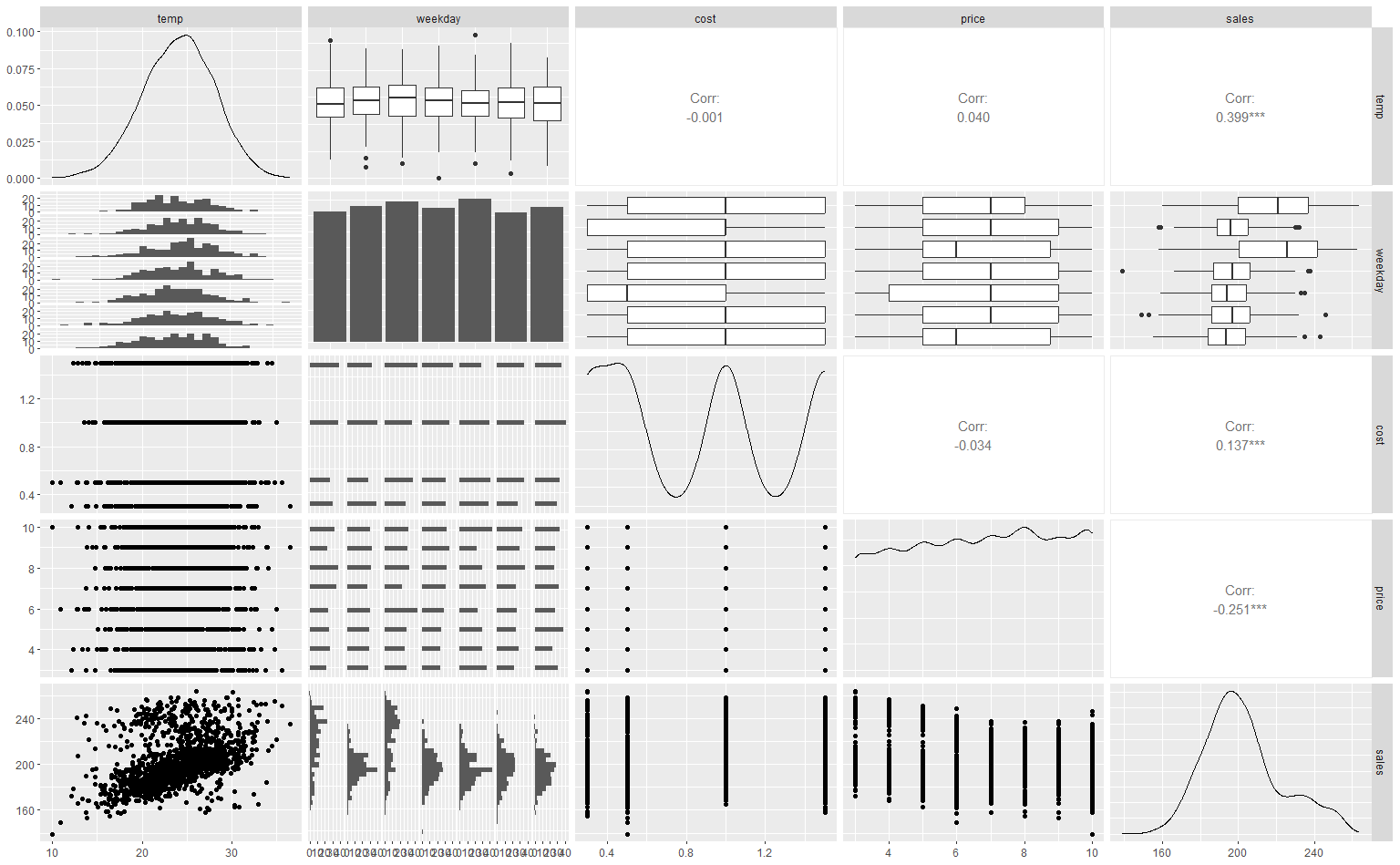
icecream %>% datasummary_skim()| Unique | Missing Pct. | Mean | SD | Min | Median | Max | Histogram | |
|---|---|---|---|---|---|---|---|---|
| temp | 200 | 0 | 24.1 | 4.0 | 10.0 | 24.2 | 36.5 | 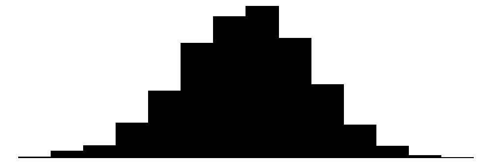 |
| cost | 4 | 0 | 0.9 | 0.5 | 0.3 | 1.0 | 1.5 | 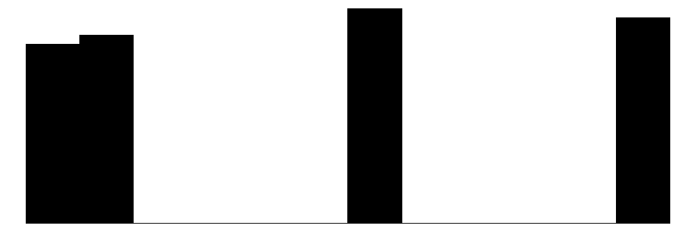 |
| price | 8 | 0 | 6.6 | 2.3 | 3.0 | 7.0 | 10.0 | 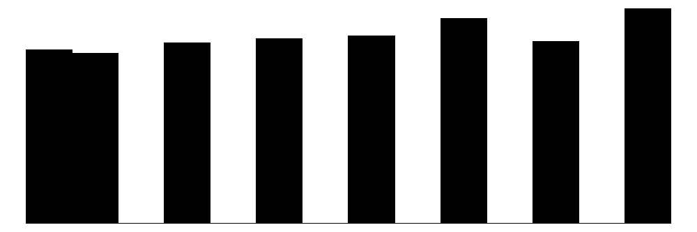 |
| sales | 108 | 0 | 202.4 | 21.0 | 139.0 | 199.0 | 264.0 |  |
| weekday | N | % | ||||||
| Sun | 206 | 13.7 | ||||||
| Tue | 215 | 14.3 | ||||||
| Sat | 222 | 14.8 | ||||||
| Wed | 212 | 14.1 | ||||||
| Fri | 226 | 15.1 | ||||||
| Mon | 205 | 13.7 | ||||||
| Thu | 214 | 14.3 |
1.3 Fit the model with an interaction between temperature and
Built a regression model with an interaction terms between prices, weekdays and temperatures.
fit1 <- lm(log(sales) ~ temp * price * weekday, icecream)
parameters(fit1)
Parameter | Coefficient | SE | 95% CI
------------------------------------------------------------------------
(Intercept) | 5.58 | 0.05 | [ 5.47, 5.68]
temp | 5.25e-03 | 2.19e-03 | [ 0.00, 0.01]
price | -0.02 | 7.95e-03 | [-0.04, 0.00]
weekday [Tue] | -0.45 | 0.08 | [-0.60, -0.30]
weekday [Sat] | -6.30e-03 | 0.08 | [-0.16, 0.14]
weekday [Wed] | -0.39 | 0.08 | [-0.54, -0.24]
weekday [Fri] | -0.46 | 0.07 | [-0.60, -0.32]
weekday [Mon] | -0.57 | 0.08 | [-0.72, -0.42]
weekday [Thu] | -0.40 | 0.07 | [-0.54, -0.25]
temp × price | -1.17e-03 | 3.25e-04 | [ 0.00, 0.00]
temp × weekday [Tue] | 3.16e-04 | 3.19e-03 | [-0.01, 0.01]
temp × weekday [Sat] | 3.19e-04 | 3.07e-03 | [-0.01, 0.01]
temp × weekday [Wed] | -2.29e-03 | 3.22e-03 | [-0.01, 0.00]
temp × weekday [Fri] | 7.56e-04 | 2.99e-03 | [-0.01, 0.01]
temp × weekday [Mon] | 5.30e-03 | 3.11e-03 | [ 0.00, 0.01]
temp × weekday [Thu] | -2.00e-03 | 3.01e-03 | [-0.01, 0.00]
price × weekday [Tue] | -8.46e-03 | 0.01 | [-0.03, 0.01]
price × weekday [Sat] | -2.08e-03 | 0.01 | [-0.02, 0.02]
price × weekday [Wed] | -0.02 | 0.01 | [-0.04, 0.00]
price × weekday [Fri] | -8.18e-03 | 0.01 | [-0.03, 0.01]
price × weekday [Mon] | 1.47e-03 | 0.01 | [-0.02, 0.02]
price × weekday [Thu] | -0.02 | 0.01 | [-0.04, 0.00]
(temp × price) × weekday [Tue] | 2.43e-03 | 4.64e-04 | [ 0.00, 0.00]
(temp × price) × weekday [Sat] | 9.15e-05 | 4.39e-04 | [ 0.00, 0.00]
(temp × price) × weekday [Wed] | 2.94e-03 | 4.59e-04 | [ 0.00, 0.00]
(temp × price) × weekday [Fri] | 2.43e-03 | 4.40e-04 | [ 0.00, 0.00]
(temp × price) × weekday [Mon] | 2.03e-03 | 4.49e-04 | [ 0.00, 0.00]
(temp × price) × weekday [Thu] | 3.00e-03 | 4.47e-04 | [ 0.00, 0.00]
Parameter | t(1472) | p
-------------------------------------------------
(Intercept) | 104.01 | < .001
temp | 2.40 | 0.017
price | -2.56 | 0.010
weekday [Tue] | -5.77 | < .001
weekday [Sat] | -0.08 | 0.934
weekday [Wed] | -4.99 | < .001
weekday [Fri] | -6.36 | < .001
weekday [Mon] | -7.49 | < .001
weekday [Thu] | -5.44 | < .001
temp × price | -3.59 | < .001
temp × weekday [Tue] | 0.10 | 0.921
temp × weekday [Sat] | 0.10 | 0.917
temp × weekday [Wed] | -0.71 | 0.478
temp × weekday [Fri] | 0.25 | 0.801
temp × weekday [Mon] | 1.70 | 0.089
temp × weekday [Thu] | -0.67 | 0.506
price × weekday [Tue] | -0.75 | 0.453
price × weekday [Sat] | -0.19 | 0.847
price × weekday [Wed] | -1.85 | 0.065
price × weekday [Fri] | -0.76 | 0.446
price × weekday [Mon] | 0.13 | 0.893
price × weekday [Thu] | -2.05 | 0.041
(temp × price) × weekday [Tue] | 5.24 | < .001
(temp × price) × weekday [Sat] | 0.21 | 0.835
(temp × price) × weekday [Wed] | 6.40 | < .001
(temp × price) × weekday [Fri] | 5.52 | < .001
(temp × price) × weekday [Mon] | 4.53 | < .001
(temp × price) × weekday [Thu] | 6.70 | < .001performance(fit1)# Indices of model performance
AIC | AICc | BIC | R2 | R2 (adj.) | RMSE | Sigma
---------------------------------------------------------------
10742.9 | 10744.1 | 10897.0 | 0.828 | 0.825 | 0.042 | 0.0431.4 Interprete the interaction term between prices and temperature
estimate_slopes and ggpredict
# estimate_slopes(______, trend = ______, at = ______ ) %>% plot()
# ggpredict(______, terms = c(______, "temp [10, 25, 35]") ) %>% ______()
1.5 Interprete the interaction term between prices and temperature
#
#
#