AE04-01 Multiple Linear Regression

Published

June 29, 2022

Setup

library(tidyverse)
library(wooldridge)
library(modelsummary)
library(GGally)
library(parameters)
library(performance)
library(see)
library(patchwork)
library(ggeffects)

ggplot2::theme_set(ggplot2::theme_bw())

knitr::opts_chunk$set(
  fig.width = 12,
  fig.asp = 0.618,
  out.width = "100%"
)

Goals

Fit multiple linear regression;
Display and interpret regression summary;
Compute fitted values and residuals;

Data

We use data from (Blackburn and Neumark, 1992) on wage determinants. Variables present are:

\(wage\) - monthly earnings in USD;
\(educ\) - years of education;
\(exper\) - years of experiences;
\(black\) - dummy variable representing individuals which are not Caucasian;

See: Blackburn, M. and Neumark, D. (1992) Unobserved Ability, Efficiency Wages, and Interindustry Wage Differentials. The Quarterly Journal of Economics , Vol. 107, No. 4. Oxford University Press (OUP). p. 1421-1436

wage_dta <- 
    wooldridge::wage2 %>% 
    as_tibble() %>% 
    select(wage, educ, exper, black)

Ex. 1. Glimpse at the data

# __________(_____)

Compute a new variables caucasian that takes values “yes” and “no” for each person depending on the values of the variable black.

# wage_dta <-
#   _____ %>%
#   mutate(_____ = ifelse(black, "no", "yes"),
#          caucasian = as.factor(caucasian))
# glimpse(_____)

Ex. 1.2. Descriptive statistics

Use function datasummary_skim() from the package modelsummary.

# library(_________)
# _________(wage_dta)

Ex. 2.3. Visual data inspection

We inspect data visually by building a grid of scatter plots using GGally::ggpairs()

# library(_________)
# _________(wage_dta)

Add parameter aes(colour = caucasian) to ggpairs().

What is the difference compare to the previous plot?

# ggpairs(_________, _________)

Ex. 2. Fit regressions

Dependent variable is wage, independent are: educ, exper and black

# fit1 <- lm(____ ~ ____ + ____ + ____, data = ____)
# fit1

Ex. 2.1. Print regression results

# fit1

Ex. 3 Regression summary

# summary(______)

Interpret the coefficients:

Ex. 2.1 Regression summary using `parameters::parameters()`

Check help on ?parameters::parameters

# library(________)
# ________(________)

Ex. 2.2. Goodness of fit using `performance::performance()`

Check help on ?performance::performance

# library(________)
# performance(________)

Ex. 4. Fitted

# fitted_vector <- fitted(________)
# fitted_vector[1:20]

Ex. 5. Residuals

# resid_vector <- resid(________)
# resid_vector[1:20]

Ex. 6. Residuals vs fitted plot

Use function plot(). Put fitted as an x argument and residuals as y.

# plot(x = _____, ___ = ________)

Ex. 6.1 Residuals vs fitted using `check_model` from `performance` package

See: ?performance::check_model

# check_model(fit1, check = "linearity")

Ex. 7 Predicting values using regression

We can compute predicted values based on the regression results for arbitrary values of \(X\). See: ?predict

First, we need to make a table the \(X\) variables for which we want compute the predicted value.

Variables names in table should match the variables in the regression.

Let us predict wage for a person with 0 years of education, 0 experience, when he/she is white.

# pred1 <-
#   tibble(educ = 0,
#          exper = 0,
#          black = 0)
# predict(fit1, pred1)

The same when the person is black.

# pred2 <-
#   tibble(educ = c(0, 0),
#          exper = c(0, 0),
#          black = c(0, 1)
#   )
# predict(fit1, pred2)

Ex 7.1 Writing predicted values to a data frame

Use mutate to mutate new variable in a data frame:

# pred3 <-
#   tibble(educ = c(0, 0, 10),
#          exper = c(0, 0, 25),
#          black = c(0, 1, 1)
#   )
# 
# pred3 %>% 
#   mutate(predicted = predict(fit1, pred3))

Ex 7.2 Visual inspection of predicted values

We can use function ggeffects::ggpredict(), check help.

# library(ggeffects)
# ggpredict(fit1, term = "educ")

We can also plot this effects using plot after ggpredict

# ggpredict(fit1, term = "educ") %>% ________()

Compute predicted values for a different independent variable and a dummy variable

# ggpredict(fit1, term = c("________", "________")) 
# ________(________, term = c("________", "________")) %>% plot()

Solutions

Code

library(tidyverse)
library(wooldridge)

wage_dta <- 
    wooldridge::wage2 %>% 
    as_tibble() %>% 
    select(wage, educ, exper, black)
glimpse(wage_dta)

Rows: 935
Columns: 4
$ wage  <int> 769, 808, 825, 650, 562, 1400, 600, 1081, 1154, 1000, 930, 921, …
$ educ  <int> 12, 18, 14, 12, 11, 16, 10, 18, 15, 12, 18, 14, 15, 16, 16, 10, …
$ exper <int> 11, 11, 11, 13, 14, 14, 13, 8, 13, 16, 8, 9, 4, 7, 9, 17, 6, 19,…
$ black <int> 0, 0, 0, 0, 0, 1, 0, 0, 0, 0, 0, 0, 0, 0, 0, 0, 0, 0, 0, 0, 0, 0…

Code

wage_dta <-
  wage_dta %>%
  mutate(caucasian = ifelse(black, "no", "yes"),
         caucasian = as.factor(caucasian))
glimpse(wage_dta)

Rows: 935
Columns: 5
$ wage      <int> 769, 808, 825, 650, 562, 1400, 600, 1081, 1154, 1000, 930, 9…
$ educ      <int> 12, 18, 14, 12, 11, 16, 10, 18, 15, 12, 18, 14, 15, 16, 16, …
$ exper     <int> 11, 11, 11, 13, 14, 14, 13, 8, 13, 16, 8, 9, 4, 7, 9, 17, 6,…
$ black     <int> 0, 0, 0, 0, 0, 1, 0, 0, 0, 0, 0, 0, 0, 0, 0, 0, 0, 0, 0, 0, …
$ caucasian <fct> yes, yes, yes, yes, yes, no, yes, yes, yes, yes, yes, yes, y…

Code

library(modelsummary)
datasummary_skim(wage_dta)

	Unique (#)	Mean	SD	Min	Median	Max
wage	449	957.9	404.4	115.0	905.0	3078.0
educ	10	13.5	2.2	9.0	12.0	18.0
exper	22	11.6	4.4	1.0	11.0	23.0
black	2	0.1	0.3	0.0	0.0	1.0

Code

library(GGally)
ggpairs(wage_dta)

`stat_bin()` using `bins = 30`. Pick better value with `binwidth`.
`stat_bin()` using `bins = 30`. Pick better value with `binwidth`.
`stat_bin()` using `bins = 30`. Pick better value with `binwidth`.
`stat_bin()` using `bins = 30`. Pick better value with `binwidth`.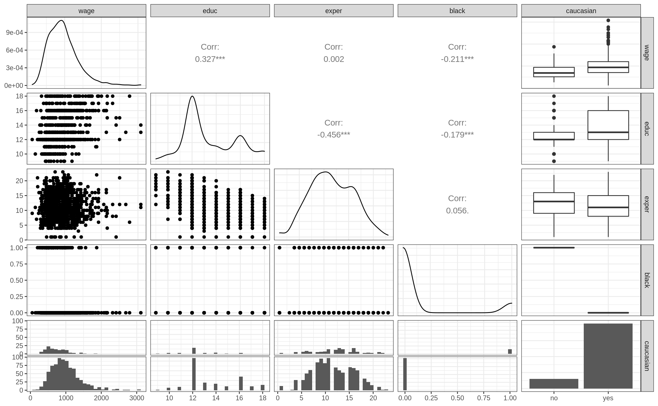

Code

ggpairs(wage_dta, aes(colour = caucasian))

Warning in cor(x, y): the standard deviation is zero

Warning in cor(x, y): the standard deviation is zero

Warning in cor(x, y): the standard deviation is zero

Warning in cor(x, y): the standard deviation is zero

Warning in cor(x, y): the standard deviation is zero

Warning in cor(x, y): the standard deviation is zero

`stat_bin()` using `bins = 30`. Pick better value with `binwidth`.
`stat_bin()` using `bins = 30`. Pick better value with `binwidth`.
`stat_bin()` using `bins = 30`. Pick better value with `binwidth`.
`stat_bin()` using `bins = 30`. Pick better value with `binwidth`.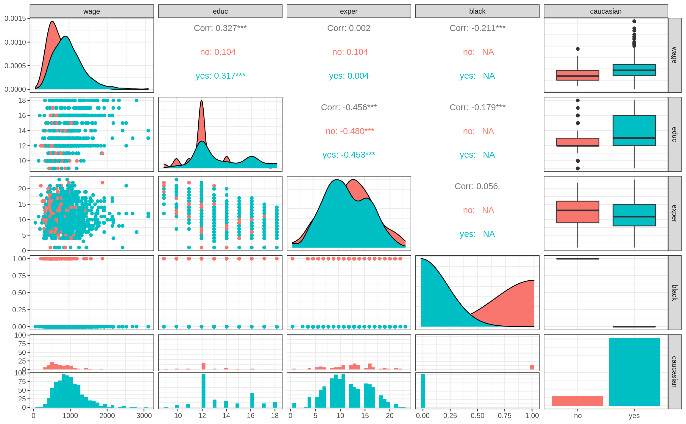

Code

fit1 <- lm(wage ~ educ + exper + black, data = wage_dta)
fit1


Call:
lm(formula = wage ~ educ + exper + black, data = wage_dta)

Coefficients:
(Intercept)         educ        exper        black  
    -170.23        70.77        17.18      -183.98

Code

summary(fit1)


Call:
lm(formula = wage ~ educ + exper + black, data = wage_dta)

Residuals:
    Min      1Q  Median      3Q     Max 
-923.57 -250.05  -35.42  195.94 2139.28 

Coefficients:
            Estimate Std. Error t value Pr(>|t|)    
(Intercept) -170.225    107.893  -1.578    0.115    
educ          70.769      6.313  11.210  < 2e-16 ***
exper         17.178      3.124   5.499 4.92e-08 ***
black       -183.984     36.948  -4.980 7.59e-07 ***
---
Signif. codes:  0 '***' 0.001 '**' 0.01 '*' 0.05 '.' 0.1 ' ' 1

Residual standard error: 371.6 on 931 degrees of freedom
Multiple R-squared:  0.1583,    Adjusted R-squared:  0.1556 
F-statistic: 58.35 on 3 and 931 DF,  p-value: < 2.2e-16

Code

library(parameters)
parameters(fit1)

Parameter   | Coefficient |     SE |             95% CI | t(931) |      p
-------------------------------------------------------------------------
(Intercept) |     -170.23 | 107.89 | [-381.97,   41.52] |  -1.58 | 0.115 
educ        |       70.77 |   6.31 | [  58.38,   83.16] |  11.21 | < .001
exper       |       17.18 |   3.12 | [  11.05,   23.31] |   5.50 | < .001
black       |     -183.98 |  36.95 | [-256.49, -111.47] |  -4.98 | < .001


Uncertainty intervals (equal-tailed) and p-values (two-tailed) computed
  using a Wald t-distribution approximation.

Code

library(performance)
performance(fit1)

# Indices of model performance

AIC       |       BIC |    R2 | R2 (adj.) |    RMSE |   Sigma
-------------------------------------------------------------
13725.631 | 13749.834 | 0.158 |     0.156 | 370.785 | 371.581

Code

fitted_vector <- fitted(fit1)
fitted_vector[1:20]

        1         2         3         4         5         6         7         8 
 867.9558 1292.5693 1009.4937  902.3111  848.7198 1018.5808  760.7732 1241.0364 
        9        10        11        12        13        14        15        16 
1114.6179  953.8440 1241.0364  975.1384  960.0191 1082.3209 1116.6762  829.4838 
       17        18        19        20 
 994.3744  934.6080  889.2502  902.3111

Code

resid_vector <- resid(fit1)
resid_vector[1:20]

         1          2          3          4          5          6          7 
 -98.95581 -484.56934 -184.49366 -252.31109 -286.71981  381.41917 -160.77325 
         8          9         10         11         12         13         14 
-160.03642   39.38214   46.15599 -311.03642  -54.13838  -60.01910  235.67906 
        15         16         17         18         19         20 
 675.32378  128.51619  365.62562  -84.60801  -59.25017 -431.31109

Code

plot(x = fitted_vector, y = resid_vector)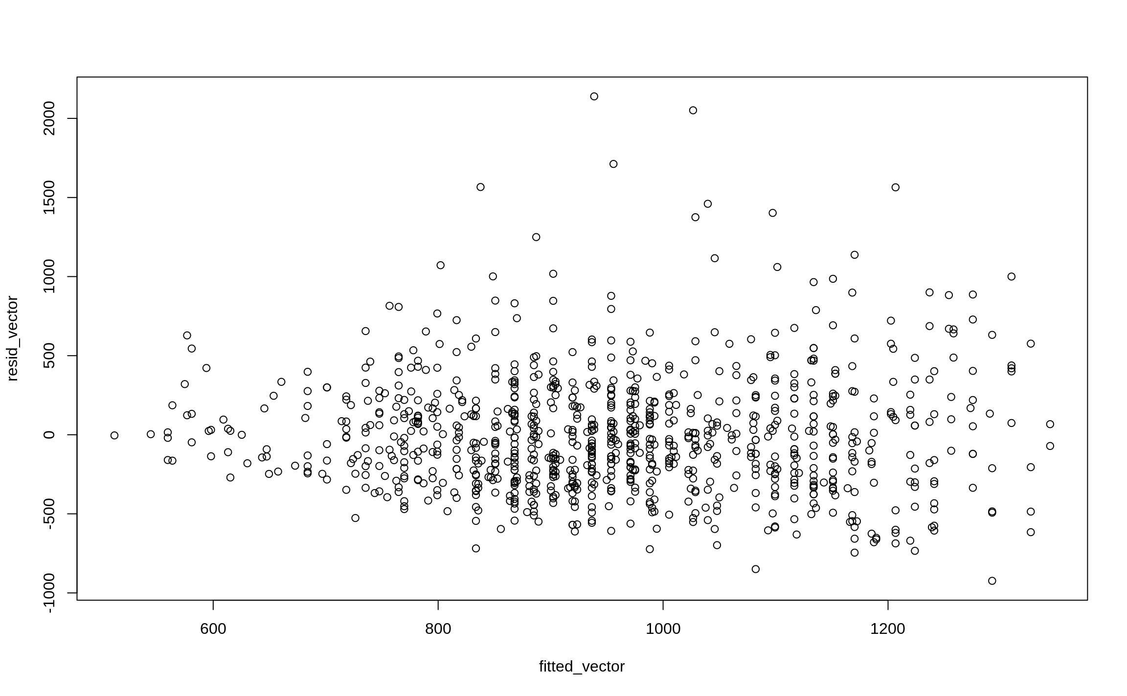

Code

check_model(fit1, check = "linearity")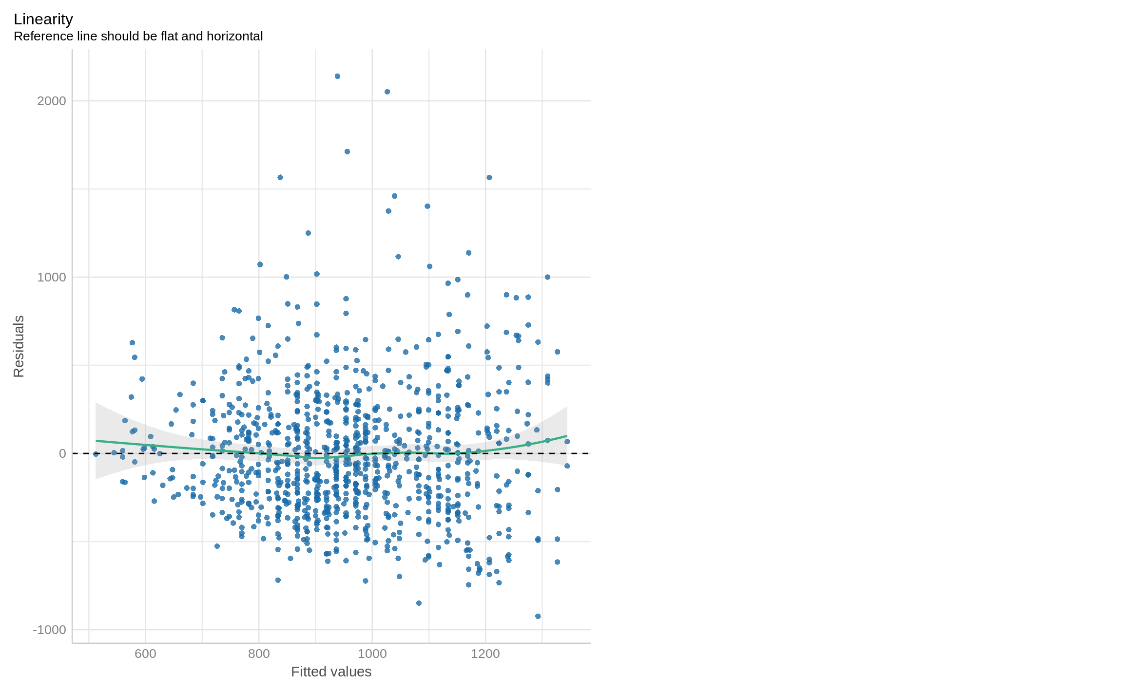

Code

pred1 <-
 tibble(educ = 0,
        exper = 0,
        black = 0)
predict(fit1, pred1)

        1 
-170.2253

Code

pred2 <-
  tibble(educ = c(0, 0),
         exper = c(0, 0),
         black = c(0, 1)
  )
predict(fit1, pred2)

        1         2 
-170.2253 -354.2089

Code

pred3 <-
  tibble(educ = c(0, 0, 10),
         exper = c(0, 0, 25),
         black = c(0, 1, 1)
  )
pred3 %>% 
  mutate(predicted = predict(fit1, pred3))

# A tibble: 3 × 4
   educ exper black predicted
  <dbl> <dbl> <dbl>     <dbl>
1     0     0     0     -170.
2     0     0     1     -354.
3    10    25     1      783.

Code

library(ggeffects)

ggpredict(fit1, term = "educ")

# Predicted values of wage

educ | Predicted |             95% CI
-------------------------------------
   9 |    655.65 | [ 591.81,  719.49]
  10 |    726.42 | [ 673.67,  779.16]
  11 |    797.19 | [ 754.83,  839.55]
  12 |    867.96 | [ 834.59,  901.32]
  14 |   1009.49 | [ 983.63, 1035.36]
  15 |   1080.26 | [1050.16, 1110.37]
  16 |   1151.03 | [1112.96, 1189.11]
  18 |   1292.57 | [1233.79, 1351.35]

Adjusted for:
* exper = 11.00
* black =  0.00

Code

ggpredict(fit1, term = "educ") %>% plot()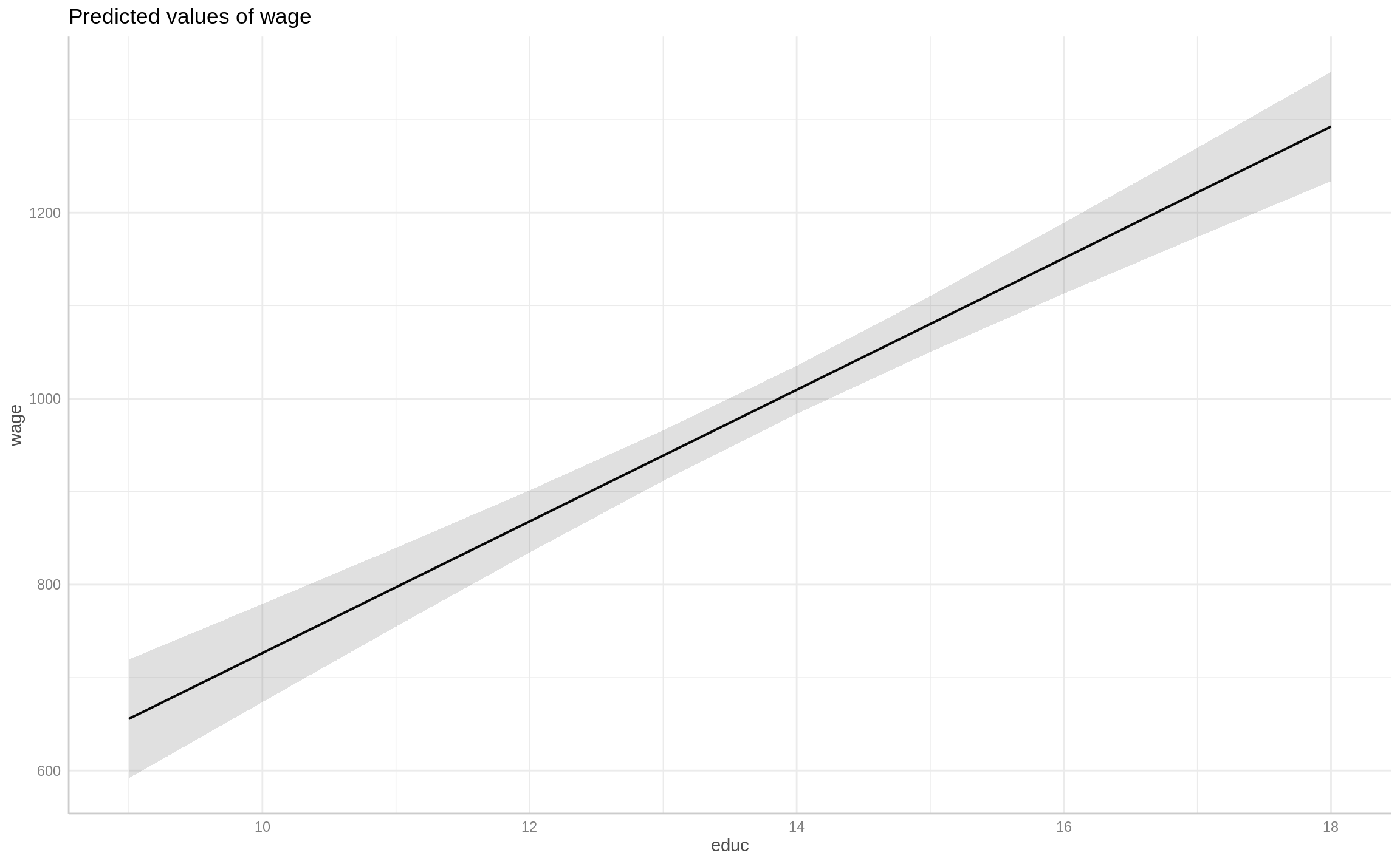

Code

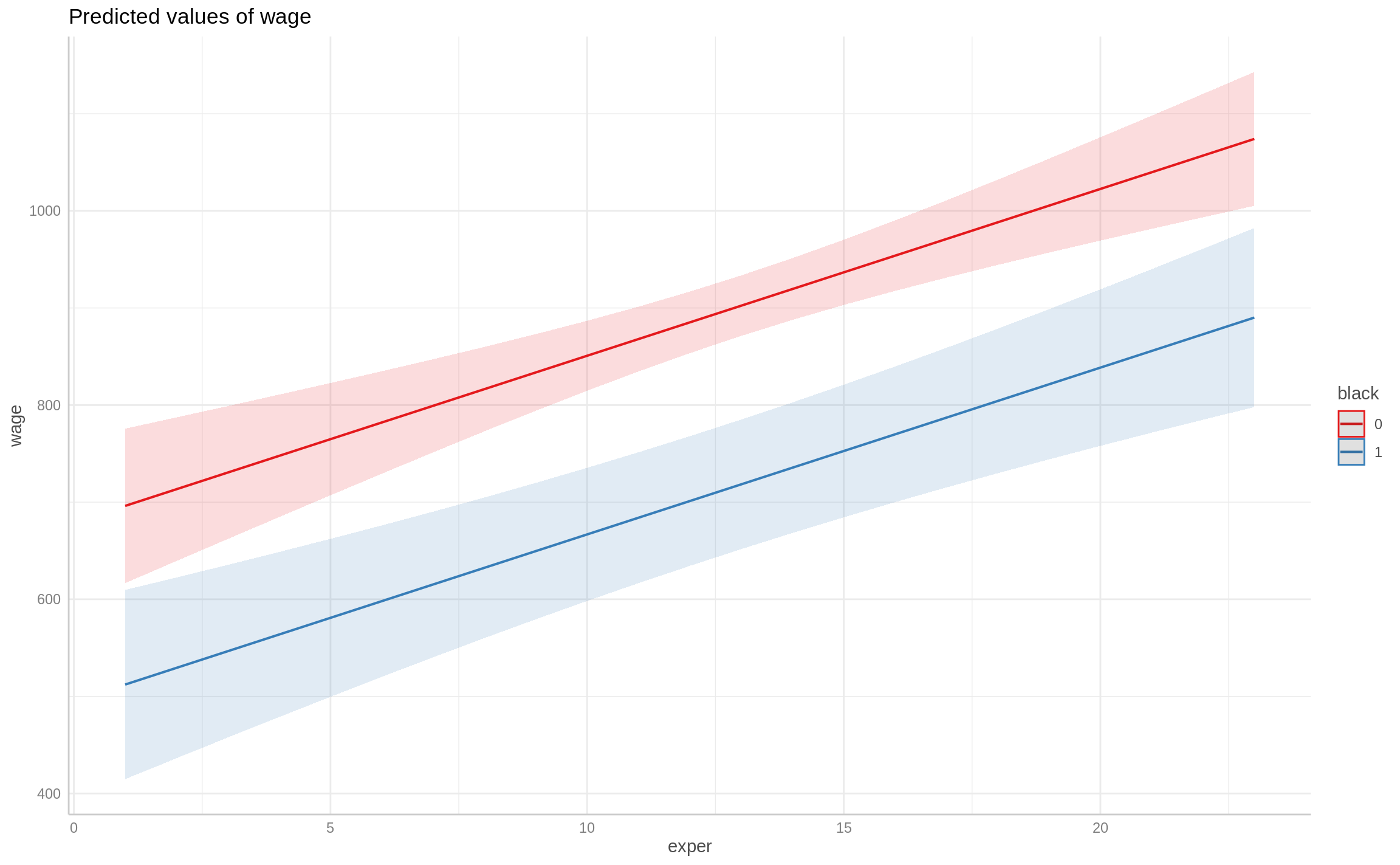
ggpredict(fit1, term = c("exper", "black"))

# Predicted values of wage

# black = 0

exper | Predicted |             95% CI
--------------------------------------
    1 |    696.18 | [ 616.64,  775.72]
    5 |    764.89 | [ 707.08,  822.70]
    8 |    816.42 | [ 772.95,  859.90]
   12 |    885.13 | [ 853.45,  916.82]
   16 |    953.84 | [ 917.55,  990.14]
   23 |   1074.09 | [1005.16, 1143.02]

# black = 1

exper | Predicted |           95% CI
------------------------------------
    1 |    512.20 | [414.77, 609.62]
    5 |    580.91 | [499.60, 662.22]
    8 |    632.44 | [560.06, 704.82]
   12 |    701.15 | [634.39, 767.91]
   16 |    769.86 | [700.03, 839.69]
   23 |    890.10 | [797.94, 982.26]

Adjusted for:
* educ = 12.00

Code

ggpredict(fit1, term = c("exper", "black")) %>% plot()

Setup

Goals

Data

Ex. 1. Glimpse at the data

Ex. 1.2. Descriptive statistics

Ex. 2.3. Visual data inspection

Ex. 2. Fit regressions

Ex. 2.1. Print regression results

Ex. 3 Regression summary

Ex. 2.1 Regression summary using parameters::parameters()

Ex. 2.2. Goodness of fit using performance::performance()

Ex. 4. Fitted

Ex. 5. Residuals

Ex. 6. Residuals vs fitted plot

Ex. 6.1 Residuals vs fitted using check_model from performance package

Ex. 7 Predicting values using regression

Ex 7.1 Writing predicted values to a data frame

Ex 7.2 Visual inspection of predicted values

Solutions

Ex. 2.1 Regression summary using `parameters::parameters()`

Ex. 2.2. Goodness of fit using `performance::performance()`

Ex. 6.1 Residuals vs fitted using `check_model` from `performance` package