Instrumental Variable
MP223 - Applied Econometrics Methods for the Social Sciences
Eduard Bukin
Refresh
What is the ceteris paribus?
What is the Selection Bias?
How is Selection Bias different from the OVB?
What is long, short and auxiliary regression?
What is the OVB formula?
Why is selection bias causing a problem?
Return to schooling ans Selection bias
Does more years of schooling cause higher wages?
Jacob Mincer first try to quantify the return to schooling (see Mincer 1974) by estimating the log of annual earning (\(\ln Y_i\)) as a function of years of education (\(s_i\)) and potential work experience (\(x_i\)) in the following fashion:
\[ \ln Y_i = \alpha + \rho s_i + \beta_1 x_i + \beta_2 x^{2}_i + \varepsilon_i \qquad(1)\]
Answer to the following questions:
Why is experience introduced in a quadratic form?
Prove that omitting experience causes bias to years of education.
Show bias of the excluded experience
- Write down long, short, auxiliary regression and the OVB formula.
- Short: \(\ln Y_i = \alpha^S + \rho^{S} s_i + \varepsilon_i^S\)
- Long: \(\ln Y_i = \alpha + \rho^L s_i + \beta_1 x_i + \varepsilon_i\)
- Auxiliary: \(x_i = \delta_0 + \delta_{xs} s_i + \upsilon_i\)
- OVB formula: \(\text{OVB} = \delta_{xs} \times \rho^L\)
- Hypothesize about \(\delta_{xs}\) and \(\rho^L\)
- Relationship between education and income: \(\rho^L_i > 0\)
- Relationship between experience and education: \(\delta_{xs} < 0\)
- \(\text{OVB} = \delta_{xs} \times \rho^L = \{\delta_{xs} > 0 \} \times \{ \rho < 0 \} \Longrightarrow \text{OVB} < 0\)
- Excluding \(x_i\) cases bias of the return to education;
- It reduces the estimated level of \(\rho^S\) either to lower value or below zero. It could also make it insignificantly different from zero.
Is ceteris paribus fulfilled in the Mincer’s equation?
- Is control for potential experience sufficient for ceteris to be paribus? At a given experience level, are more- and less-educated workers equally able and diligent? 1
- We may rewrite Equation 1 in the way that it incorporates ability:
\[Y_i = \alpha + \rho s_i + \gamma A^{'}_{i} + \varepsilon_i \qquad(2)\]
- where \(A^{'}_{i}\) vector of control variables such as ability, experience and that we desire to have in order to ensure the unbiased estimates of \(\rho\).
- Omitting ability causes a Selection bias: \(\rho^{S} = \rho + \underbrace{\delta_{A^{'} s} \times \gamma}_{\text{ability bias}}\)
Solutions to the selection bias
Randomized trials/experiments (Joshua D. Angrist and Pischke 2009, Ch 1-2.; Joshua D. Angrist and Pischke 2014, Ch. 1);
Regression analysis (Joshua D. Angrist and Pischke 2009, Ch 3.; Joshua D. Angrist and Pischke 2014, Ch. 2);
- Multiple regression (M. J. Wooldridge 2020, Ch. 3);
- Panel regression (M. J. Wooldridge 2020, Ch. 13-14; Croissant and Millo 2018; J. M. Wooldridge 2010)
- Other regressions: binary outcome (logit/probit), censored data (tobit), truncated data, count data (poisson regression), quantile regression …
Instrumental variables
- IV (2SLS, GMM) (Joshua D. Angrist and Pischke 2009, Ch. 4.; Joshua D. Angrist and Pischke 2014, Ch. 3);
- LATE – Local average treatment effect
- Sample selection models, Heckman … (M. J. Wooldridge 2020, Ch. 17; Cameron and Trivedi 2005, Ch. 11-27)
DID - Difference in Difference;
RDD - Regression Discontinuity Design;
Endogeneity
Is another terminology for the selection bias problem
Definition
- Consider following LONG and SHORT models:
\[Y_i = \alpha + \rho s_i + \gamma A^{'}_{i} + \varepsilon_i \\ Y_i = \alpha^S + \rho^S s_i + \varepsilon^{S}_i\]
- where \(s_i\) is a causal variable of interest and \(A^{'}_{i}\) is the vector of control variables that we desire to have in order to ensure unbiased estimates of \(\rho\);
Confusing definition of endogeneity:
- Variable \(s_i\) is endogenous if it correlates with the error terms \(\varepsilon^{S}_i\) : \(Cov(s_i, \varepsilon^{S}_i) \neq 0\)
Definition (cont.)
In practice, endogeneity means that
- variation in the independent variable \(s_i\) (years of education) are not “random” as compared to the variation in the dependent variable \(Y_i\), but rather
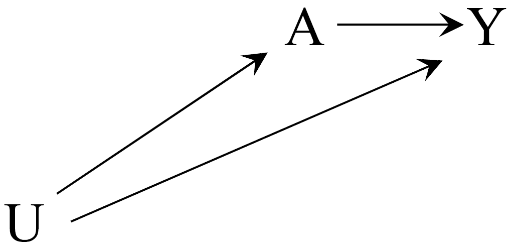
- an external process \(U\) affects variation in both \(s_i\) and \(Y_i\);
- thus, \(s_i\) is endogenous to \(Y_i\);
If variance of \(s_i\) is truly independent of \(Y_i\), \(s_i\) is exogenous.
Causes of endogeneity
Omitted Variable Bias
Measurement Error
Simultaneity
Omitted Variable Bias
Long model: \(Y_i = \alpha + \rho s_i + \gamma A^{'}_{i} + \varepsilon_i\)
Short model: \(Y_i = \alpha^S + \rho^S s_i + \varepsilon^{S}_i\)
If \(s_i\) and \(A_i\) are correlated, we can assume a linear relationship between them:
\[ A_i = \delta_0 + \delta_1 s_i + \upsilon_i \]
\[ \Rightarrow Y_i = \alpha + \rho s_i + \gamma (\delta_0 + \delta_1 A_i + \upsilon_i) + \varepsilon_i \]
\[ = \underbrace{(\alpha + \gamma \delta_0)}_{\alpha^S} + \underbrace{(\rho + \gamma \delta_1)}_{\rho^S} s_i + \underbrace{(\varepsilon_i + \gamma \upsilon_i)}_{\varepsilon_i^S} \]
Omitted Variable Bias: visually
Measurement error
We estimate a long model: \(Y_i = \alpha + \beta s^*_i + e_i \\\) ,
- but \(s^*_i\) is unavailable, we only have \(s_i = s^*_i + m_i\) instead
- \(m_i\) is a systematic measurement error
- \(E[m_i] =0\) and \(Cov(s^*_i, m_i) = Cov(e_i, m_i) = 0\).
Desired coefficient \(\beta = \frac{Cov(Y_i, s_i)}{Var(s_i)}\)
But with the erroneous data, we estimate biased coefficient \(\beta_b\)
\[ \beta_b = \frac{Cov(Y_i, s_i)}{Var(s_i)} = \frac{Cov(a+\beta s^*_i + e_i, s^*_i + m_i)}{Var(s_i)} \\ = \frac{\beta \cdot Cov(s^*_i, s^*_i)}{Var(s_i)} = \beta \frac{Var(s^{*}_i)}{Var(s_i)} \]
- (see Joshua D. Angrist and Pischke 2014, Ch. 6)
Simultaneity
Simultaneity occurs if at least two variables are jointly determined.
- A typical case is when observed outcomes are the result of separate behavioral mechanisms that are coordinated in an equilibrium.
The prototypical case is a system of demand and supply equations:
- \(D(p)\) = how high would demand be if the price was set to \(p\)?
- \(S(p)\) = how high would supply be if the price was set to \(p\)?
Number of police people and the crime rate.
(see M. J. Wooldridge 2020, Ch. 17) for more details on the problem and solutions.
Solutions to endogeneity
There are same five “lethal” weapons against endogeneity as there were against the selection bias:
- Randomized Control Trials / Experiments
- Regression
- Instrumental variable
- Difference in difference
- Regression discontinuity design
Instrumental Variable
Recall the short (\(Y_i = \alpha^S + \rho^S s_i + \varepsilon^{S}_i\)) and long (\(Y_i = \alpha + \rho s_i + \gamma A^{'}_{i} + \varepsilon_i\)) models.
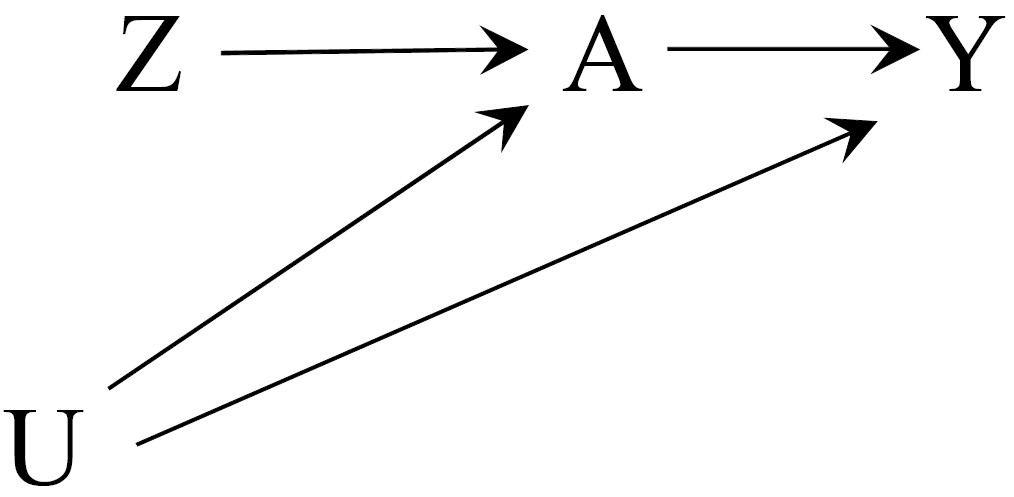
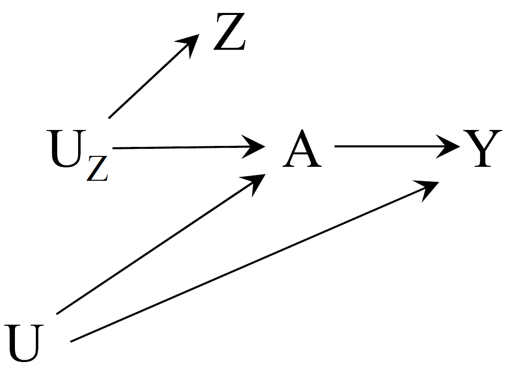
Instrumental Variable is another variable \(Z_i\) that satisfy:
Relevance condition:
- \(Z_i\) has a causal effect on \(s_i\) (or strong association with (see Hernán and Robins 2020, 194));
Exclusion restriction:
- \(Z_i\) does not affect \(Y_i\) directly, except through its potential effect on \(s_i\);
Independence assumption:
- \(Z_i\) is randomly assigned or “as good as randomly assigned”, same as
- \(Z_i\) is unrelated to the omitted variables \(A^{'}_i\), same as
- \(Z_i\) and \(Y_i\) do not share any common causes
Important
(see Joshua D. Angrist and Pischke 2014 Ch. 3 and 6; Joshua D. Angrist and Pischke 2009, Ch. 4.; Hernán and Robins 2020, Ch. 16; J. M. Wooldridge 2010, Ch. 8; Söderbom, Teal, and Eberhardt 2014, Ch. 11)
Instrumental Variable visually (1)
Instrumental Variable visually (2)
IV regression using 2SLS (1)
Imagine that we have:
- long model: \(Y_i = \alpha + \rho s_i + \gamma A^{'}_{i} + \varepsilon_i\) ;
- short model: \(Y_i = \alpha^S + \rho^S s_i + \varepsilon^{S}_i\) ;
- with endogenous \(s_i\), and
- a valid instrument \(Z_i\)
Estimate the first stage: \(s_i = \pi_0 + \pi_1 Z_i + nu_i\)
Substitute \(s_i\) with the fitted values from the first stage \(\hat{s_i}\)
Estimate the second stage: \(Y_i = \alpha^{IV} + \rho^{IV} \hat{s_i} + \varepsilon^{IV}_i\)
where
- \(\hat{s_i}\) are the fitted values from the first stage
- \(\rho^{IV}\) is the causal effect of interest from stage two that is asymptotically equal to \(\rho\) , the true effect of interest (\(\rho^{IV} \asymp \rho\))
IV intuition using 2SLS (2)
wg1 <- wooldridge::wage2 %>% as_tibble() %>%
  filter(if_all(c(wage, educ, exper, meduc), ~!is.na(.)))
#
ols <-  lm(log(wage) ~ educ + exper + I(exper^2), wg1)
#
first_stage <- lm(educ ~ meduc + exper + I(exper^2), wg1)
#
second_stage <- lm(log(wage) ~ educ_fit + exper + I(exper^2),
                   wg1 %>% mutate(educ_fit = fitted(first_stage)))
# A tibble: 9 × 4
parameter OLS `First stage` `Second stage`
<chr> <chr> <chr> <chr>
1 (Intercept) "5.4864*** (0.1308)" "12.7886*** (0.4575)" "4.3947*** (0.35…
2 educ "0.0802*** (0.0068)" "" ""
3 meduc "" "0.2199*** (0.0227)" ""
4 educ_fit "" "" "0.1518*** (0.02…
5 exper "0.0147 (0.0143)" "-0.0455 (0.0684)" "0.0170 (0.0151)"
6 I(exper^2) "0.0003 (0.0006)" "-0.0070* (0.0029)" "0.0010 (0.0007)"
7 N "857" "857" "857"
8 R-sq. adj. "0.1387" "0.2898" "0.0482"
9 F Statistics (df) "47*** (3)" "117*** (3)" "15*** (3)" Pitfalls of the IV
Consistency and unbiasedness
IV estimates are not unbiased, but they are consistent (Joshua D. Angrist and Krueger 2001).
Unbiasedness means the estimator has a sampling distribution centered on the parameter of interest in a sample of any size, while
Consistency only means that the estimator converges to the population parameter as the sample size grows.
Note
Researchers that use IV should aspire to work with large samples.
- No statistical tests is available for checking the consistency
Bad instruments (1)
\(Z_i\) that does not satisfy any of the Relevance condition, Exclusion restriction and Independence assumption;
\(Z_i\) that correlate with omitted variable (OV):
They result into much greater upwards shifting bias compare to the OLS;
For example the weather in Brazil and supply price and demand quantity of coffee:
weather shifts the supply curve, it is random, thus it seems as a plausible instrument for price in the demand model
the weather in Brazil determines supply expectations on futures exchange, thus, it also shifts the demand for coffee before the supply price is affected;
Bad instruments (2)
Weak instrument \(Z_i\):
When the instrument \(Z_i\) is only weakly correlates with endogenous regressor \(s_i\);
Find a better one!
Weak instrument test:
Run the first stage regression with and without the IV;
Compare the F-statistics
- If F-statistics with instrument is greater than that without by 5 of more,
- this is a sign of a strong instrument (Staiger and Stock 1997);
This test does not ensure that our instruments are independent of omitted variable \(A^{'}_i\) or \(Y_i\);
Staiger and Stock (1997)
Overidentification (1)
number of instruments \(G\) in exceeds the number of endogenous variables \(K\).
- when the IV is overidentified, estimates are biased;
- bias is proportional to \(K - G\);
- using fewer instruments therefore reduces bias;
If you have few candidates for IV and one endogenous regressor:
- select one IV for the first stage, and
- put the remaining instruments into the second stage
Overidentification (2)
Sargan’s overidentification test:
\(H_0:Cov(Z^{'}_i,\varepsilon^{IV}_i)=0\) - the covariance between the instrument and the error term is zero
\(H_1:Cov(Z^{'}_i,\varepsilon^{IV}_i)\neq0\)
Thus, by rejecting the \(H_0\), we conclude that at least one of the instruments is not valid.
Wu-Hausman test for endogeneity
Wu-Hausman test for endogeneity tests if the variable that we are worried about is indeed endogenous.
\(H_0:Cov(s_i,\varepsilon_i)=0\) - the covariance between potentially endogenous variable and the error term is zero
\(H_1:Cov(s_i,\varepsilon_i) \neq 0\)
Thus, by rejecting the \(H_0\), we conclude that there is endogeneity and there might be a need for IV.
Example 1 (cont.) wage and education
Angrist, J. D., & Krueger, A. B. (1991). Does Compulsory School Attendance Affect Schooling and Earnings? The Quarterly Journal of Economics, 106, 979–1014. https://doi.org/10.2307/2937954
Mincer regression and ability bias
Recall the Mincer’s regression Equation 1 with monthly wage (\(Y_i\)) as a function of years of education (\(s_i\)) and years of experience (\(x_i\)).
- Its’ estimations are based on the 1960th sample of 31k white man are below:
- \(\ln Y_i = \alpha + \underset{(.002)}{.070} s_i + \varepsilon_i\)
- \(\ln Y_i = \alpha + \underset{(.001)}{.107} s_i + \underset{(.001)}{.081} x_i - \underset{(.00002)}{.0012} x^{2}_i + \varepsilon_i\)
Answer to the following questions:
- Interpret education and experience regression coefficients;
- Does education matter much for a person with 30 years of experience?
Why Education is endogenous?
…
Ability bias!
Is it sufficient to use the IQ or knowledge of work index to resolve this bias?
What about creativity?
How to quantify the lottery change effect of getting a decent job?
How to measure the connections?
Where to find an IV?
Fantastic IVs and how to find them?
Use theory!!!
- human capital theory suggests that people make schooling choices by comparing the costs and benefits of alternatives.
Think and speculate:
- What is the ideal experiment that could capture the effect of schooling on education?
- What are the forces you’d like to manipulate and the factors you’d like to hold constant?
- What are the other processes that are independent of wage, but may affect schooling?
Analyze, what were/are the policies/environments that could mimic the experimental setting?
Fantastic IVs for education
- Loan policies or other subsidies that vary independently of ability or earnings potential
- Region and time variation in school construction (Duflo 2001)
- Proximity to college(Card 1994)
- Quarter of birth (Joshua D. Angrist and Krueger 1991)
- Parents education (Buckles and Hungerman 2013)
- Number of siblings
Reasoning on how researcher use theory and available observational data to approximate real experiment is called Identification strategy!
Random nature of the date of birth
Angrist, J. D., & Krueger, A. B. (1991). Does Compulsory School Attendance Affect Schooling and Earnings? The Quarterly Journal of Economics, 106, 979–1014. https://doi.org/10.2307/2937954
Identification strategy:
Policy required students to enter school in the calendar year in which they turned six years old;
Children born in the fourth quarter enter school at age 5 and 3⁄4 , while those born in the first quarter enter school at age 6 3⁄4;
Compulsory schooling laws require students to remain in school until their 16th birthdays;
Combination of school start age policies and compulsory schooling laws creates a natural experiment in which children are compelled to attend school for different lengths of time depending on their birthdays.
Average schooling by quarter of birth
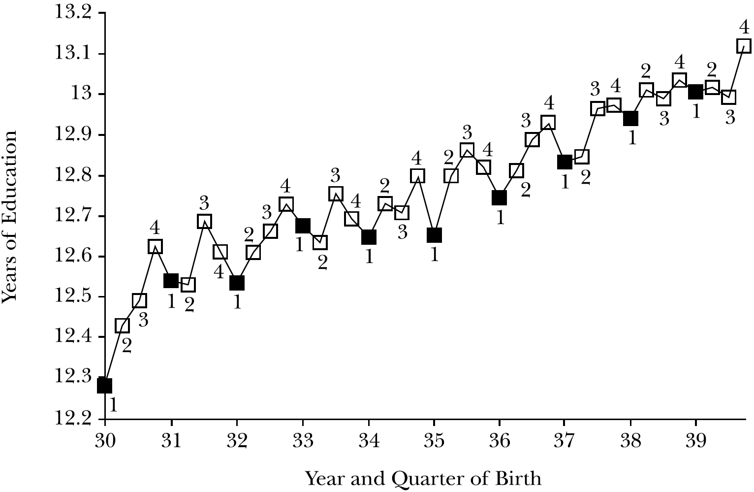
Source: (Joshua D. Angrist and Krueger 1991)
Average wage by quarter of birth
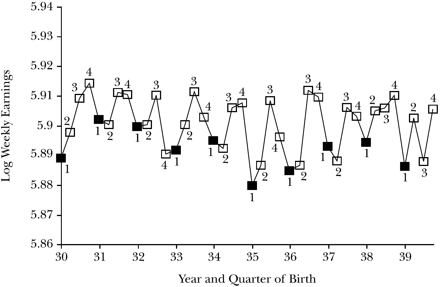
Source: (Joshua D. Angrist and Krueger 1991)
Fantastic instrumental variable:
Quarter of birth;
The intuition is:
Only a small part of variance in education (the one linked to the quarter of birth) is used to identify the return to education.
This small part of variance occurs due to random natural experiment, thus the ceteris paribus holds here.
Estimates
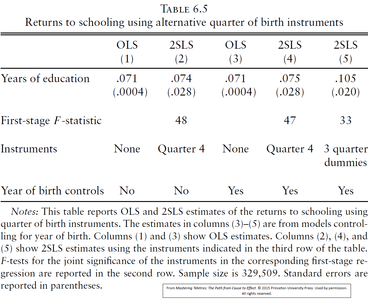
Conclusions
IV estimates are very close to the OLS;
What does it mean?
- Ability bias was small in the OLS!
Questions about questions
Research FAQs:
Before running a regression, ask the following four questions (see Joshua D. Angrist and Pischke 2009, Ch. 1)
What is the causal relationship of interest?
What is the experiment that could ideally be used to capture the causal effect of interest?
What is your identification strategy?
What is your mode of statistical inference?
FAQ 1. What is the causal relationship of interest?
FAQ 2. What is the experiment…?
Describe an ideal experiment.
Highlight the forces you’d like to manipulate and the factors you’d like to hold constant.
FUQs: fundamentally unidentified questions
Causal effect of race or gender;
- However, we can experiment with how believes about a person’s gender of race affect decisions (Bertrand and Mullainathan 2004).
Do children that start school 1 year later learn more in the primary school?
- Because older kinds are in general better learners there is not counter factual.
- However, it is possible to establish this school starting effect on adults (Black, Devereux, and Salvanes 2008).
FAQ 3. What is your identification strategy?
Identification strategy
is the manner in which a researcher uses observational data (i.e., data not generated by a randomized trial) to approximate a real experiment (Joshua D. Angrist and Krueger 1991)
Use theory!
Analyze, what were/are the policies/environments that could mimic the experimental setting?
FAQ 4. What is your mode of statistical inference?
describes the population to be studied,
the sample to be used,
and the assumptions made when constructing standard errors.
choose appropriate statistical methods
apply them diligently.
Example 2. The colonial origins of comparative development: An empirical investigation
(Acemoglu, Johnson, and Robinson 2001). The colonial origins of comparative development: An empirical investigation. American economic review, 91(5), 1369-1401.
Research question and the problem
What are the fundamental causes of the large differences in income per capita across countries?
with better “institutions,” more secure property rights, and less distortionary policies,
- countries invest more in physical and human capital, and
- use these factors more efficiently to
- achieve a greater level of income.
Institutions are a likely cause of income growth.
Endogeneity problem
What would the ideal experiment here?
Rich economies choose or can afford better institutions.
Economies that are different for a variety of reasons
- will differ both in their institutions and in their income per capita.
To estimate the impact of institutions on income,
- we need a source of exogenous variation in institutions.
Identification strategy
Current performance is cause by:
Current institutions, which are caused by
Early institutions, which are caused by
Settlements types during colonization, which are caused by
Settlers’ (potential) mortality or colonization risks.
OLS estimations
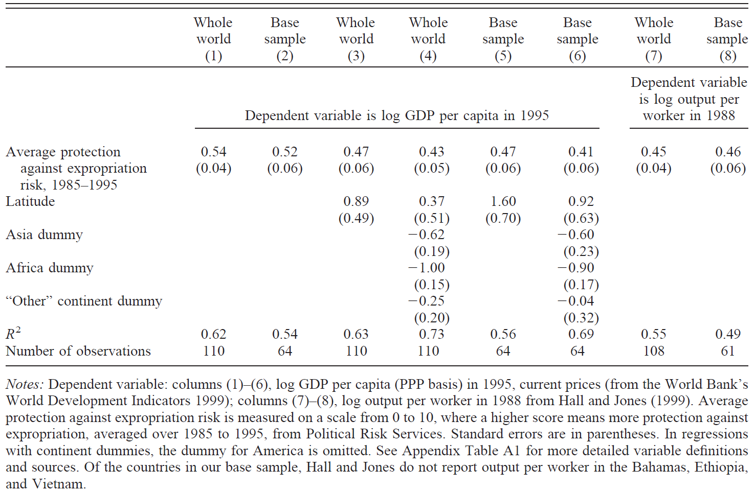
Instrumental variable
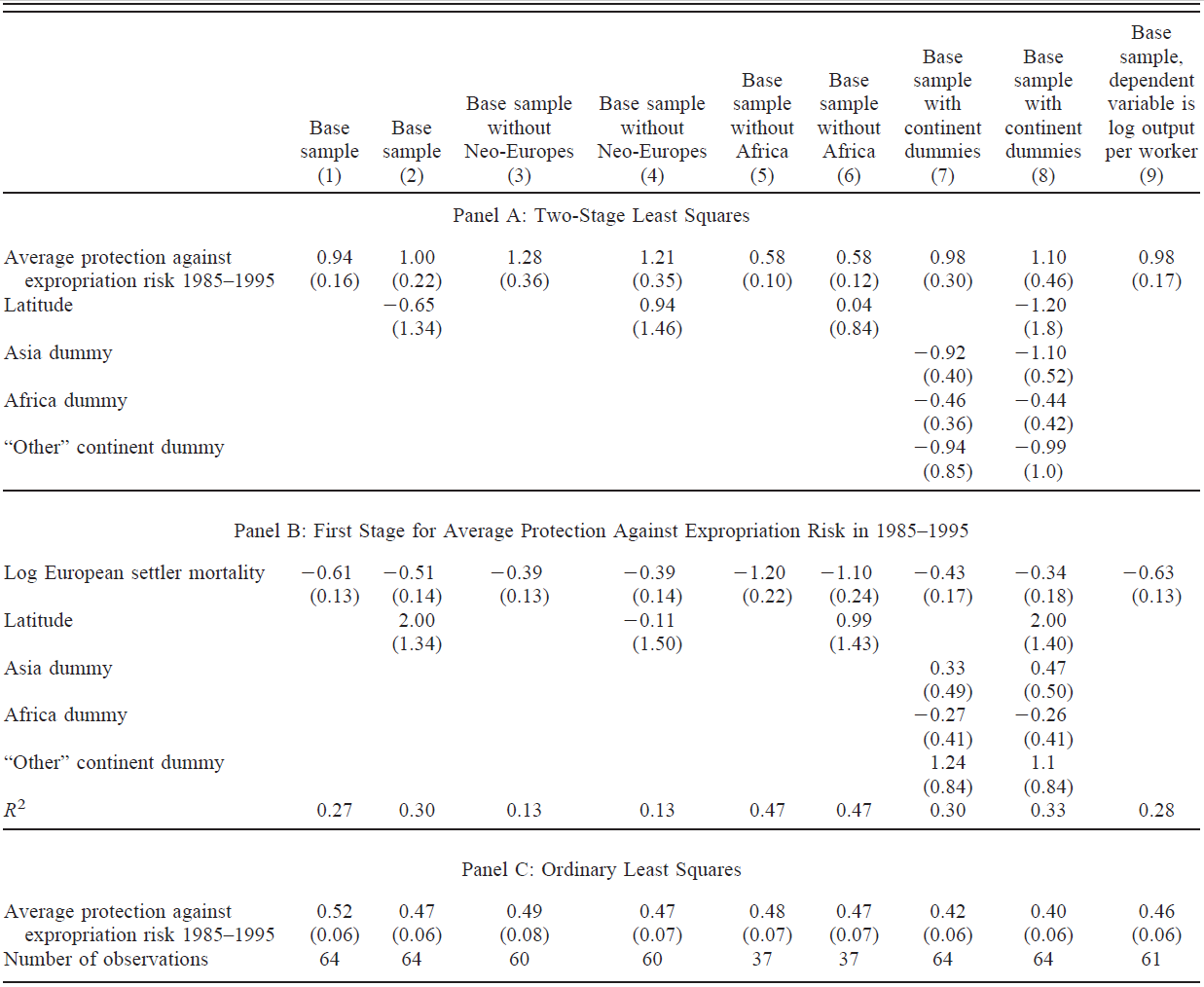
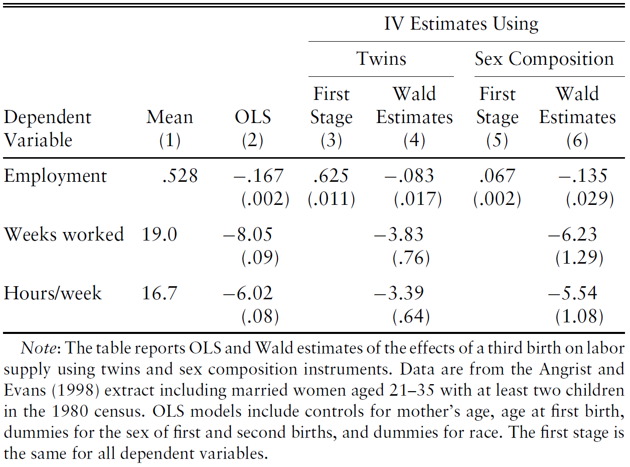
Example 3. Children and their parents’ labor supply: Evidence from exogenous variation in family size
(J. Angrist and Evans 1998) Angrist, J., & Evans, W. N. (1996). Children and their parents’ labor supply: Evidence from exogenous variation in family size.
Research question and the problem
What is the effect of additional child on women labor market participation?
Conventional wisdom:
- More children require more time therefore, women used to sacrifice own employment opportunities.
Endogeneity problem
What would the ideal experiment here?
Families without children are inappropriate counter factual
Rich families can afford more children: inappropriate counter factual
Family usually plan for having an additional children
- thus, a families with 1 children are also inappropriate counter factual
we need a source of exogenous variation in children
Identification strategy
People may plan for a second child, but they cannot plan for having a twin!
Results
References
