library(tidyverse)
library(palmerpenguins)
library(correlation)

# set default theme and larger font size for ggplot2
ggplot2::theme_set(ggplot2::theme_minimal(base_size = 16))

# set default figure parameters for knitr
knitr::opts_chunk$set(
  fig.width = 8,
  fig.asp = 0.618,
  fig.retina = 3,
  dpi = 300,
  out.width = "80%"
)
Correlation
MP223 - Applied Econometrics Methods for the Social Sciences
Eduard Bukin
R setup
Correlation
Definition of Correlation
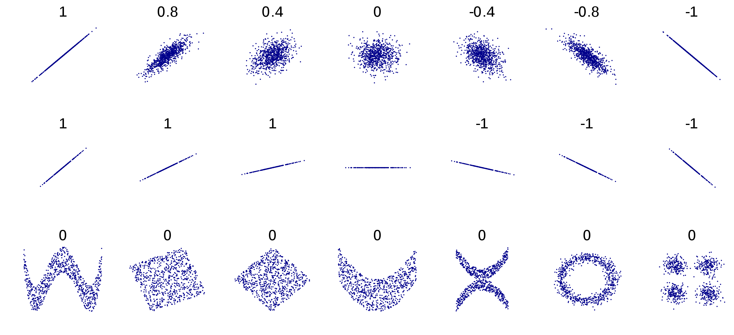
In statistics, correlation or dependence is any statistical relationship, whether causal or not, between two random variables or bivariate data.
Most common are following method of correlation:
- Pearson’s correlation
- Spearman’s rank correlation
Both, capture linear relationship.
Examples
Computation with correlation

Does Summary statistics
Documentation easystats/correlation + Source code
Learn by doing Using correlation
Key functions: correlation::correlation().
Penguins and correlation
Correlation in penguins data

The data
Rows: 344
Columns: 8
$ species           <fct> Adelie, Adelie, Adelie, Adelie, Adelie, Adelie, Adel…
$ island            <fct> Torgersen, Torgersen, Torgersen, Torgersen, Torgerse…
$ bill_length_mm    <dbl> 39.1, 39.5, 40.3, NA, 36.7, 39.3, 38.9, 39.2, 34.1, …
$ bill_depth_mm     <dbl> 18.7, 17.4, 18.0, NA, 19.3, 20.6, 17.8, 19.6, 18.1, …
$ flipper_length_mm <int> 181, 186, 195, NA, 193, 190, 181, 195, 193, 190, 186…
$ body_mass_g       <int> 3750, 3800, 3250, NA, 3450, 3650, 3625, 4675, 3475, …
$ sex               <fct> male, female, female, NA, female, male, female, male…
$ year              <int> 2007, 2007, 2007, 2007, 2007, 2007, 2007, 2007, 2007…
Scatter plot
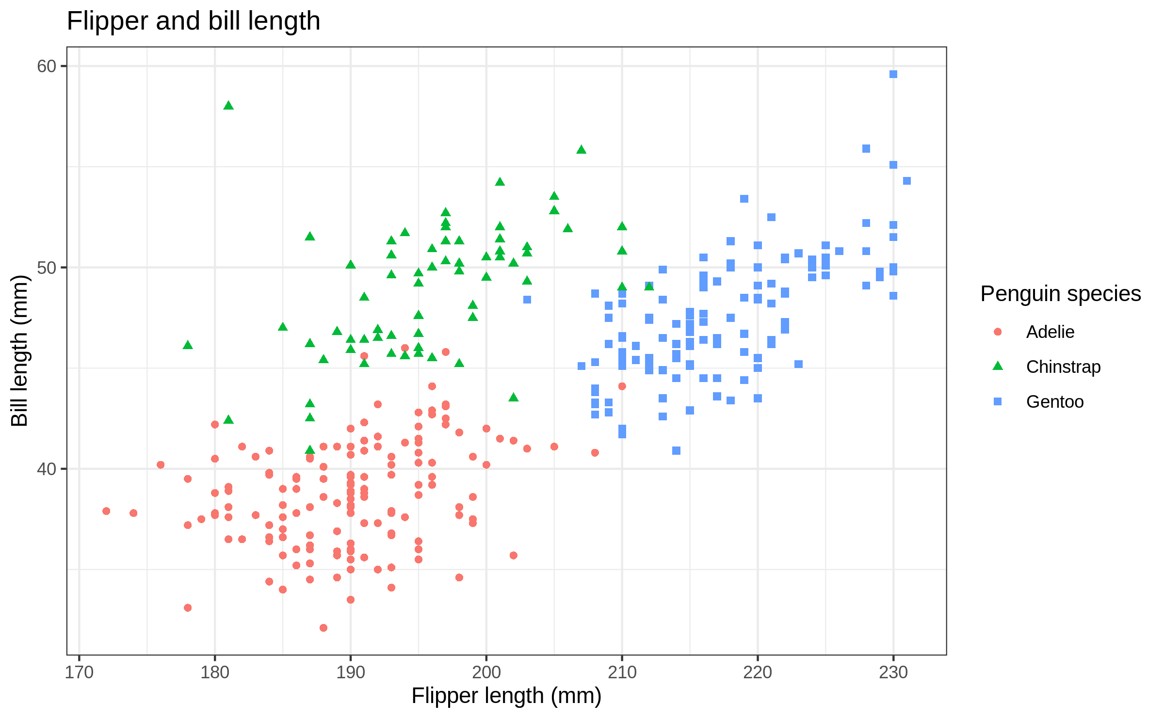
correlation() usage 1
# Correlation Matrix (pearson-method)

Parameter1        |        Parameter2 |     r |         95% CI | t(340) |         p
-----------------------------------------------------------------------------------
bill_length_mm    |     bill_depth_mm | -0.24 | [-0.33, -0.13] |  -4.46 | < .001***
bill_length_mm    | flipper_length_mm |  0.66 | [ 0.59,  0.71] |  16.03 | < .001***
bill_length_mm    |       body_mass_g |  0.60 | [ 0.52,  0.66] |  13.65 | < .001***
bill_length_mm    |              year |  0.05 | [-0.05,  0.16] |   1.01 | 0.797
bill_depth_mm     | flipper_length_mm | -0.58 | [-0.65, -0.51] | -13.26 | < .001***
bill_depth_mm     |       body_mass_g | -0.47 | [-0.55, -0.39] |  -9.87 | < .001***
bill_depth_mm     |              year | -0.06 | [-0.17,  0.05] |  -1.11 | 0.797
flipper_length_mm |       body_mass_g |  0.87 | [ 0.84,  0.89] |  32.72 | < .001***
flipper_length_mm |              year |  0.17 | [ 0.06,  0.27] |   3.17 | 0.007**
body_mass_g       |              year |  0.04 | [-0.06,  0.15] |   0.78 | 0.797

p-value adjustment method: Holm (1979)
Observations: 342
correlation() usage 2 + summary()
# Correlation Matrix (pearson-method)

Parameter         |   year | body_mass_g | flipper_length_mm | bill_depth_mm
----------------------------------------------------------------------------
bill_length_mm    |   0.05 |     0.60*** |           0.66*** |      -0.24***
bill_depth_mm     |  -0.06 |    -0.47*** |          -0.58*** |
flipper_length_mm | 0.17** |     0.87*** |                   |
body_mass_g       |   0.04 |             |                   |

p-value adjustment method: Holm (1979)
correlation() usage 3 + as_tibble()
# A tibble: 10 × 11
   Parameter1        Parameter2         r    CI  CI_low CI_high       t df_error
   <chr>             <chr>          <dbl> <dbl>   <dbl>   <dbl>   <dbl>    <int>
 1 bill_length_mm    bill_depth_… -0.235   0.95 -0.333  -0.132   -4.46       340
 2 bill_length_mm    flipper_len…  0.656   0.95  0.591   0.713   16.0        340
 3 bill_length_mm    body_mass_g   0.595   0.95  0.522   0.660   13.7        340
 4 bill_length_mm    year          0.0545  0.95 -0.0518  0.160    1.01       340
 5 bill_depth_mm     flipper_len… -0.584   0.95 -0.650  -0.509  -13.3        340
 6 bill_depth_mm     body_mass_g  -0.472   0.95 -0.550  -0.385   -9.87       340
 7 bill_depth_mm     year         -0.0604  0.95 -0.165   0.0460  -1.11       340
 8 flipper_length_mm body_mass_g   0.871   0.95  0.843   0.895   32.7        340
 9 flipper_length_mm year          0.170   0.95  0.0648  0.271    3.17       340
10 body_mass_g       year          0.0422  0.95 -0.0641  0.148    0.779      340
# … with 3 more variables: p <dbl>, Method <chr>, n_Obs <int>
Correlation in commodity prices
What commodity causes surges? (1/3)
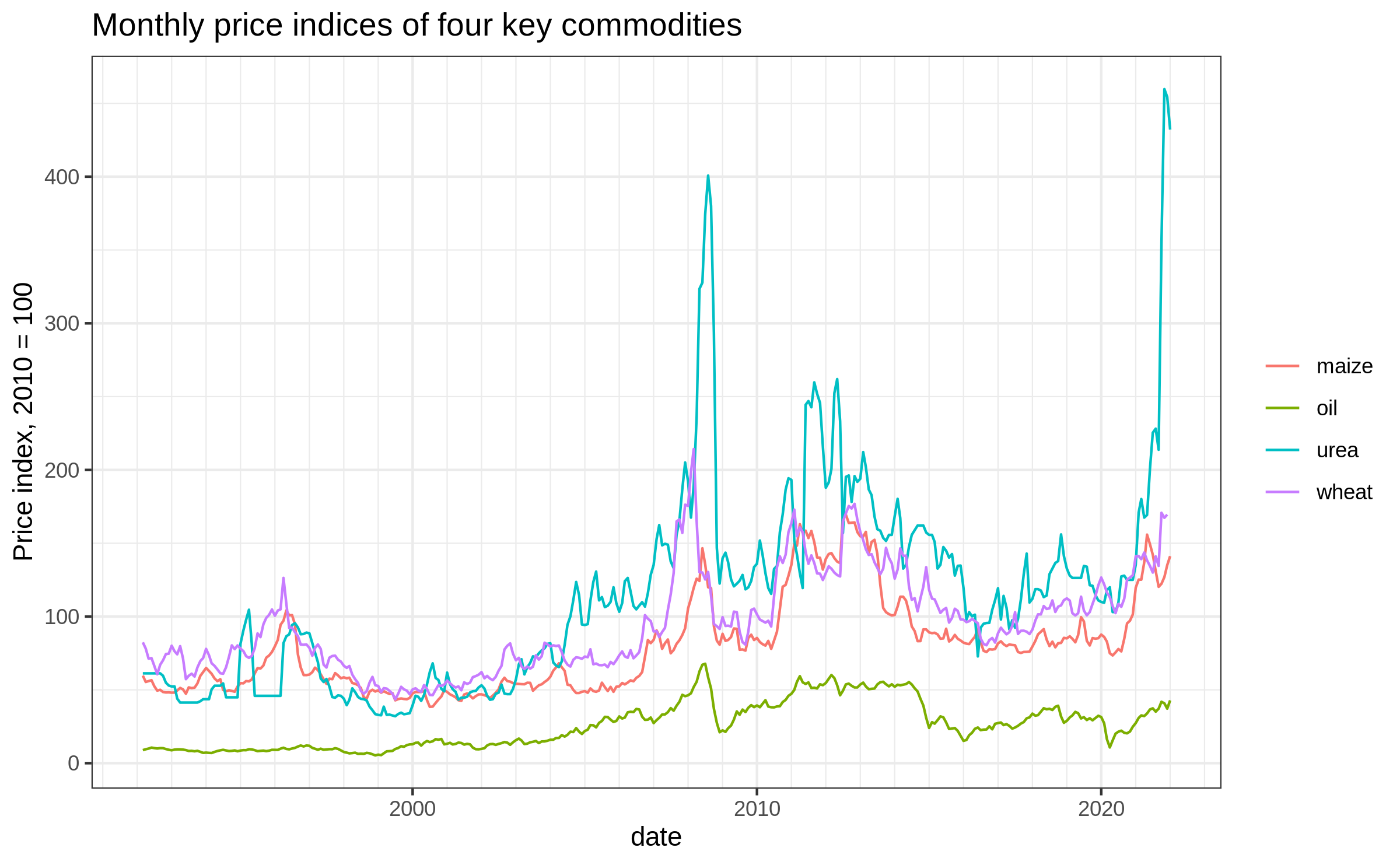
What commodity causes surges? (2/3)
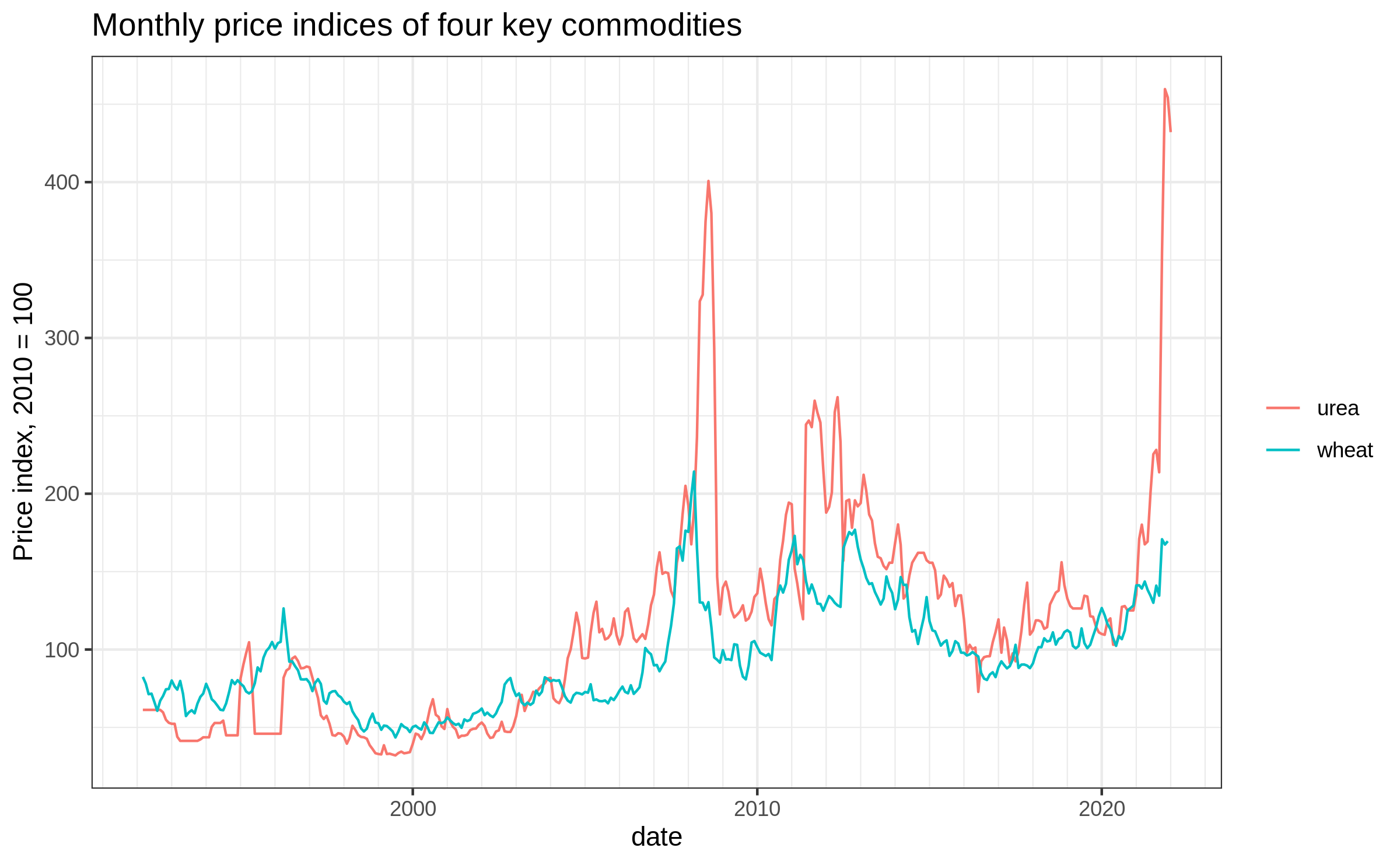
What commodity causes surges? (3/3)
Can we conclude, based on the plot, that surging prices of
ureacause thewheatprices to surge?What could be the theoretical explanation for this cause and effect relationship?
What could be the theoretical mechanism of
ureaprices effect onwheat?How can we test empirically, if there is any (co)relationship?
Prices correlation (1/2)
# Correlation Matrix (pearson-method)

Parameter   | index_wheat | index_urea | index_oil
--------------------------------------------------
index_maize |     0.89*** |    0.77*** |   0.81***
index_oil   |     0.79*** |    0.80*** |
index_urea  |     0.76*** |            |

p-value adjustment method: Holm (1979)
If we assume that theoretical causation from Urea to Wheat prices is possible!
Does high and significant correlation suggest about causal relationship?
First Difference and correlation (1/2)
# Correlation Matrix (pearson-method)

Parameter      | index_fd_wheat | index_fd_urea | index_fd_oil
--------------------------------------------------------------
index_fd_maize |        0.41*** |          0.02 |      0.25***
index_fd_oil   |           0.07 |       0.24*** |
index_fd_urea  |          -0.05 |               |

p-value adjustment method: Holm (1979)
First Difference and correlation (2/2)
First Difference removed linear trends from the data.
There might be some different chains of reaction here. For example:
Oil price may affect Urea prices as it is an important production factor
Oil price may affect maize price as it is a baleful competitor
Maize price affect wheat as they are the substitute.
Takeaway:
Correlation: linear relationship;
Does not implies causation because of no Ceteris Paribus;
- Simultaneity problem in time series.
First difference helps to remove serial trend;