Simple regression
MP223 - Applied Econometrics Methods for the Social Sciences
Eduard Bukin
R setup
# load packages
library(tidyverse)       # for data wrangling
library(alr4)            # for the data sets #
# set default theme and larger font size for ggplot2
ggplot2::theme_set(ggplot2::theme_bw())
# set default figure parameters for knitr
knitr::opts_chunk$set(
  fig.width = 8,
  fig.asp = 0.618,
  fig.retina = 3,
  dpi = 300,
  out.width = "80%"
)
Data
Pearson-Lee data
Data used is published in (Pearson and Lee 1903).
Karl Pearson collected data on over 1100 families in England in the period 1893 to 1898;
Heights of mothers
mheightand daughtersdheightwas recorded for 1375 observations.We rely on the examples of SLR in (Weisberg 2005)
Data loading and preparation
- Loading data
- Converting data frame into a
tibble()object - Renaming variables
- Glimpse of data
Code
Rows: 400
Columns: 2
$ mother_height   <dbl> 58.8, 65.4, 65.5, 63.2, 60.1, 61.2, 60.8, 63.7, 63.8, …
$ daughter_height <dbl> 62.7, 66.2, 62.8, 62.2, 65.1, 64.8, 63.4, 64.3, 62.5, …
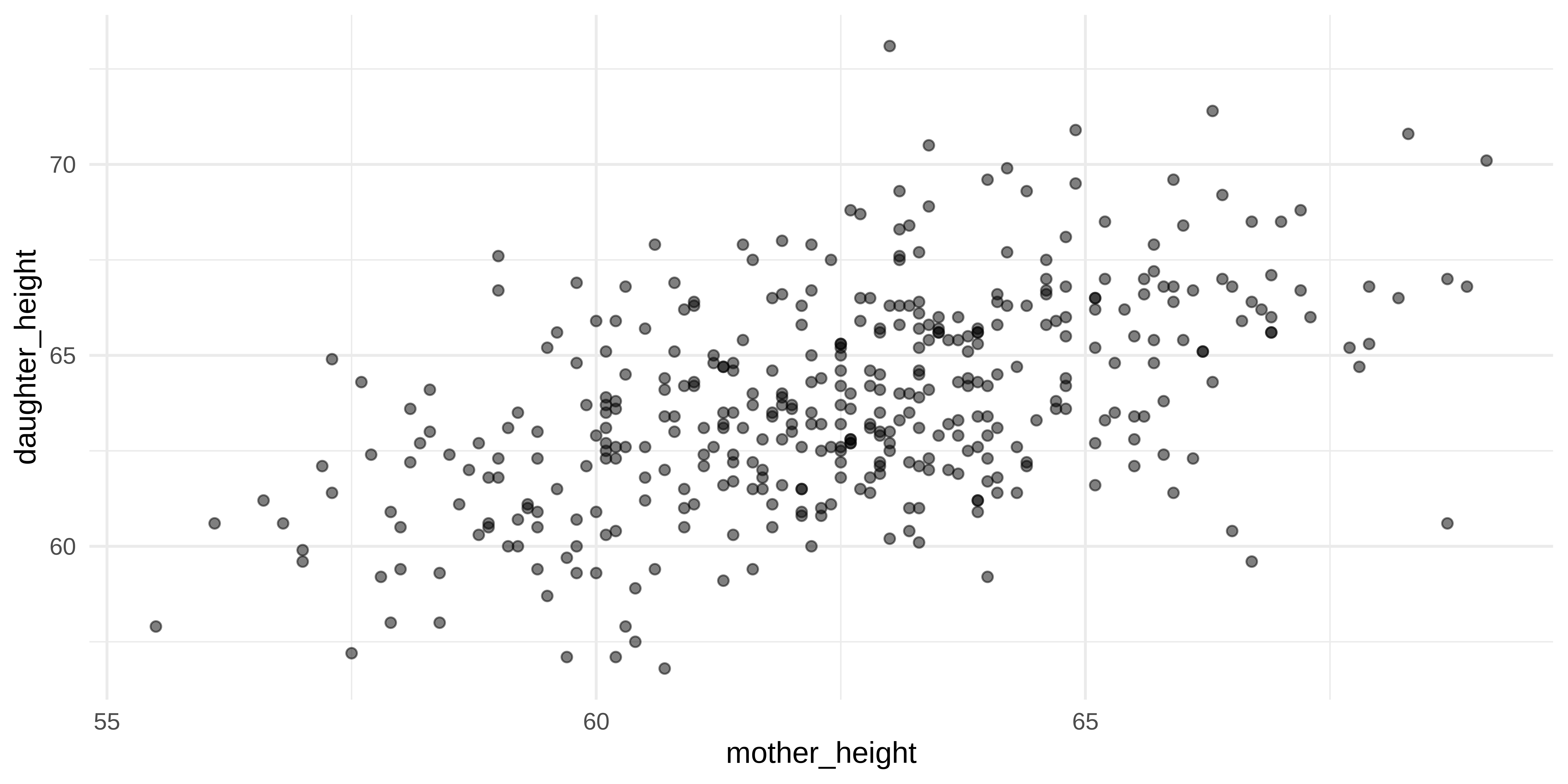
Exploring data (Scatter plot)
Simple Linear Regression
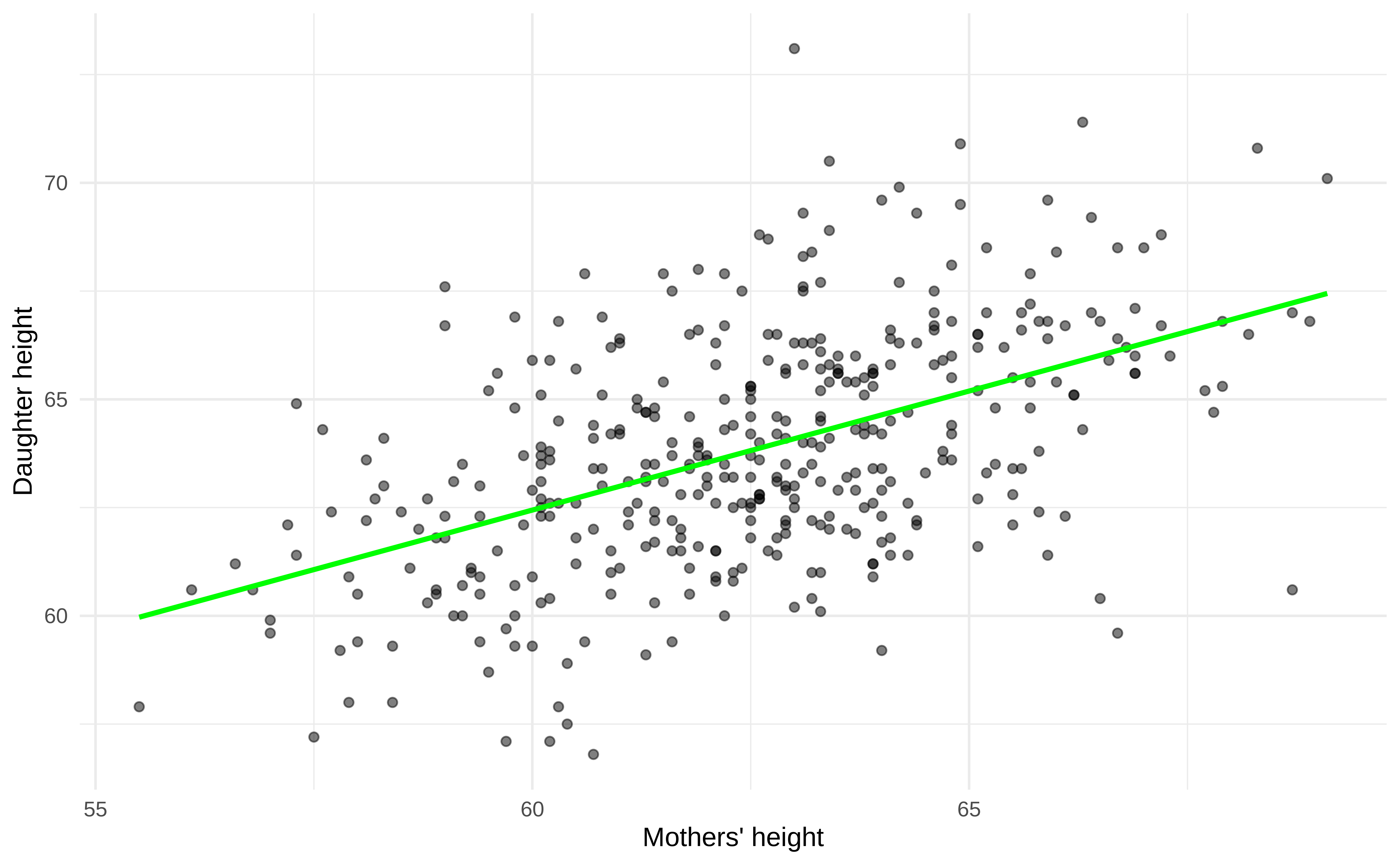
Simple regression line
Simple regression
\[\Large{Y = \beta_0 + \beta_1 X}\]
- \(Y\): dependent variable, observed values
- \(X\): independent variable
- \(\beta_1\): True slope
- \(\beta_0\): True intercept
- Note, in the population regression function, there is no error terms!
Estimated simple regression
\[\Large{\hat{Y} = \hat{\beta}_0 + \hat{\beta}_1 X}\]
- \(\hat{Y}\): fitted values, predicted values
- \(\hat{\beta}_1\): Estimated slope
- \(\hat{\beta}_0\): Estimated intercept
- No error term!
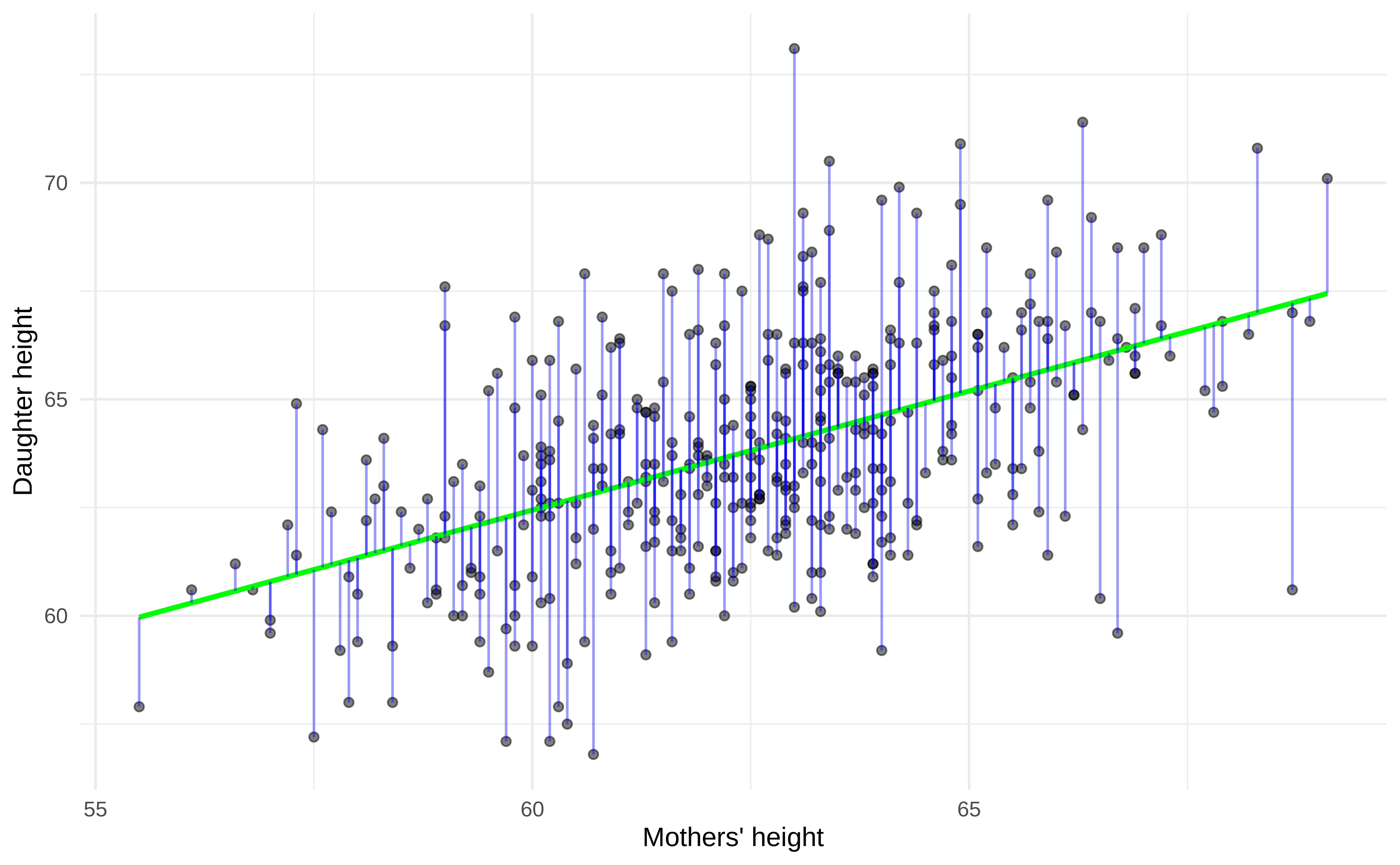
Residuals
Residuals
\(\text{residuals} \\ = \text{observed} - \text{predicted} \\ = \epsilon = Y - \hat{Y}\)
\({Y = \hat{\beta}_0 + \hat{\beta}_1 X + \epsilon}\)
\(\epsilon\) is the error term or residual
For each specific observation \(i\)
residual \(e_i = y_i - \hat{y_i}\)
squared residual \(e_i^2 = (y_i - \hat{y_i})^2\)
Ordinary Least Square (OLS)
Ordinary Least Square (OLS)
“finds” values for \(\hat{\beta}_0\) and \(\hat{\beta}_1\)
each new value of \(\hat{\beta}_0\) and \(\hat{\beta}_1\) generates new regression line;
Code
plt +
  geom_segment(
    aes(x = mother_height, xend = mother_height,
        y = daughter_height, yend = predict(fit)),
    color = "blue",
    alpha = 0.4
) +
geom_abline(intercept = 33, slope = 0.49, color = "black") +
geom_abline(intercept = 5, slope = 0.95, color = "black") +
geom_abline(intercept = 25, slope = 0.62, color = "black")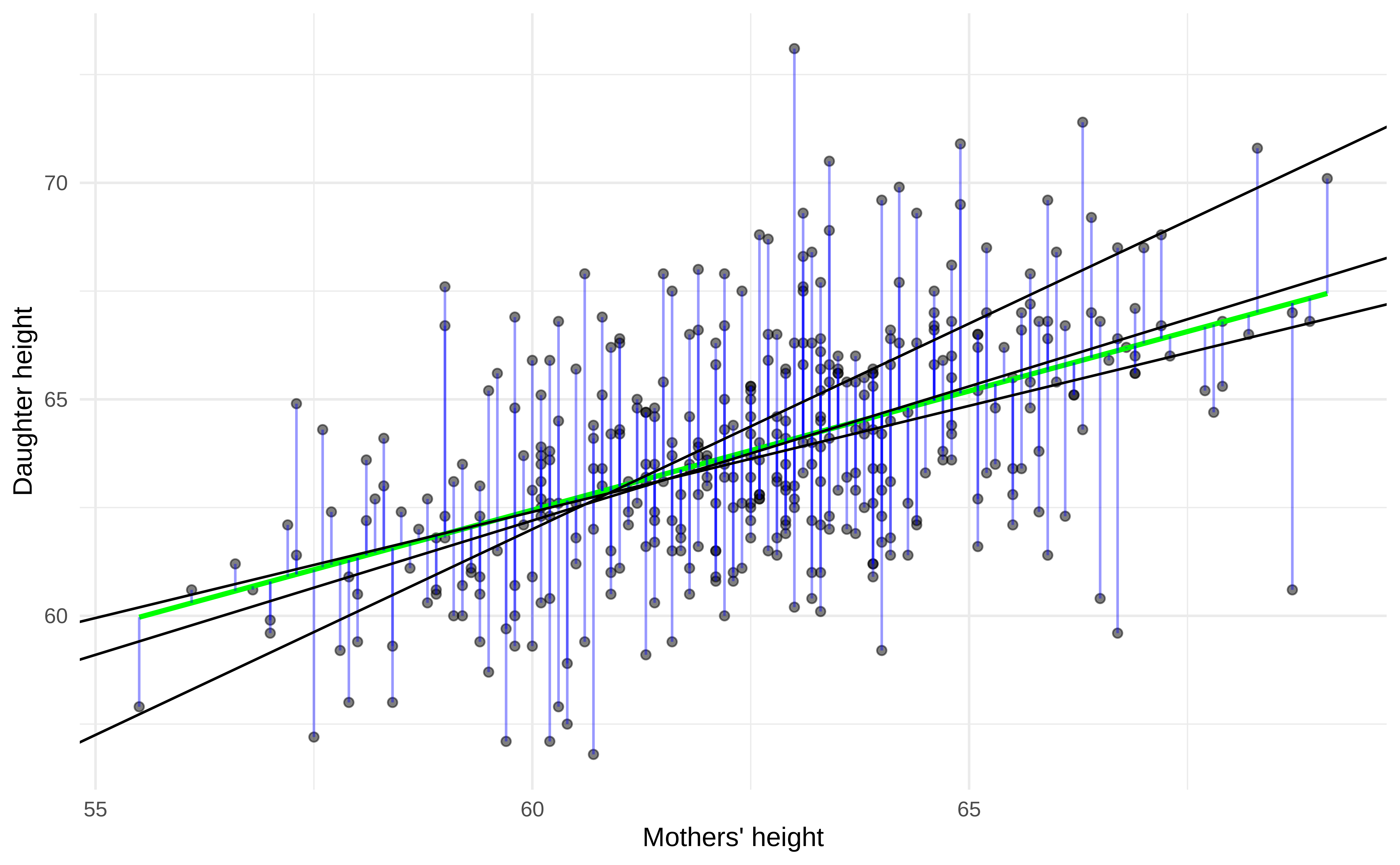
Ordinary Least Square (OLS)
the OLS finds such values of \(\hat{\beta}_0\) and \(\hat{\beta}_1\) that minimizes the sum of squared residuals:
\[ \Large{ SSR = \sum_{i}^{n}{e_i^2} = \sum_{i}^{n}{(y_i - \hat{y_i})^2} \\ = {[e_1^2 + e_2^2 + ... + e_n^2]} } \]
Properties of OLS
The regression line goes through the center of all point.
The sum of the residuals (not squared) is zero: \(\sum_{i}^n e_i = 0\)
Zero correlation between residuals and regressors \(Cov(X,\epsilon) = 0\)
Predicted value of \(Y\), when all regressors are at means \(\bar{X}\) is the mean of \(\bar{Y}\): \(E[Y|\bar{X}] = \bar{Y}\)
Interpretation
Regression coefficients
Regression summary (1/3)
Call:
lm(formula = daughter_height ~ mother_height, data = dta)

Residuals:
    Min      1Q  Median      3Q     Max
-6.6255 -1.5767 -0.0878  1.3916  9.0083

Coefficients:
              Estimate Std. Error t value Pr(>|t|)
(Intercept)   29.45511    2.91727   10.10   <2e-16 ***
mother_height  0.54979    0.04662   11.79   <2e-16 ***
---
Signif. codes:  0 '***' 0.001 '**' 0.01 '*' 0.05 '.' 0.1 ' ' 1

Residual standard error: 2.337 on 398 degrees of freedom
Multiple R-squared:  0.2589,    Adjusted R-squared:  0.2571
F-statistic: 139.1 on 1 and 398 DF,  p-value: < 2.2e-16
Regression summary (2/3)
- using
broompackage overview and source code
# A tibble: 2 × 5
  term          estimate std.error statistic  p.value
  <chr>            <dbl>     <dbl>     <dbl>    <dbl>
1 (Intercept)     29.5      2.92        10.1 1.71e-21
2 mother_height 0.550 0.0466 11.8 9.88e-28Regression summary (3/3)
- using
parameterspackage overview and source code
Parameter     | Coefficient |   SE |         95% CI | t(398) |      p
---------------------------------------------------------------------
(Intercept)   |       29.46 | 2.92 | [23.72, 35.19] |  10.10 | < .001
mother height | 0.55 | 0.05 | [ 0.46, 0.64] | 11.79 | < .001- using
performancepackage overview and source code
Intercept
Important in the context of the data.
Value of \(Y\) when all \(X\) are zero.
Slope
Marginal effect or unit change in \(Y\) on average, when \(X\) is being change by on unit, keeping all other regressors fixed.
- When mother’s height increases by 1 inch, the height of a daughter increases by \(\hat{\beta_1}\) inches, keeping other variables constant.
Residuals and Fitted values
Residuals
         1          2          3          4          5          6          7
 0.9173961  0.7887997 -2.6661790 -2.0016682  2.6026726  1.6979065  0.5178215
         8          9         10         11         12         13         14
-0.1765618 -2.0315406 -1.5917107 -5.4523061 -5.1774125  0.8022473 -1.4757112
        15         16         17         18         19         20
-3.4674550 4.0178215 -0.6813279 -3.6462641 1.8927151 -4.2860940 1 2 3 4 5 6 7
0.9173961 0.7887997 -2.6661790 -2.0016682 2.6026726 1.6979065 0.5178215
8 9 10 11 12 13 14
-0.1765618 -2.0315406 -1.5917107 -5.4523061 -5.1774125 0.8022473 -1.4757112
15 16 17 18 19 20
-3.4674550 4.0178215 -0.6813279 -3.6462641 1.8927151 -4.2860940 Fitted
       1        2        3        4        5        6        7        8
61.78260 65.41120 65.46618 64.20167 62.49733 63.10209 62.88218 64.47656
       9       10       11       12       13       14       15       16
64.53154 64.09171 62.55231 62.27741 61.39775 66.67571 62.16746 62.88218
      17       18       19       20
65.08133 65.24626 62.60728 65.68609
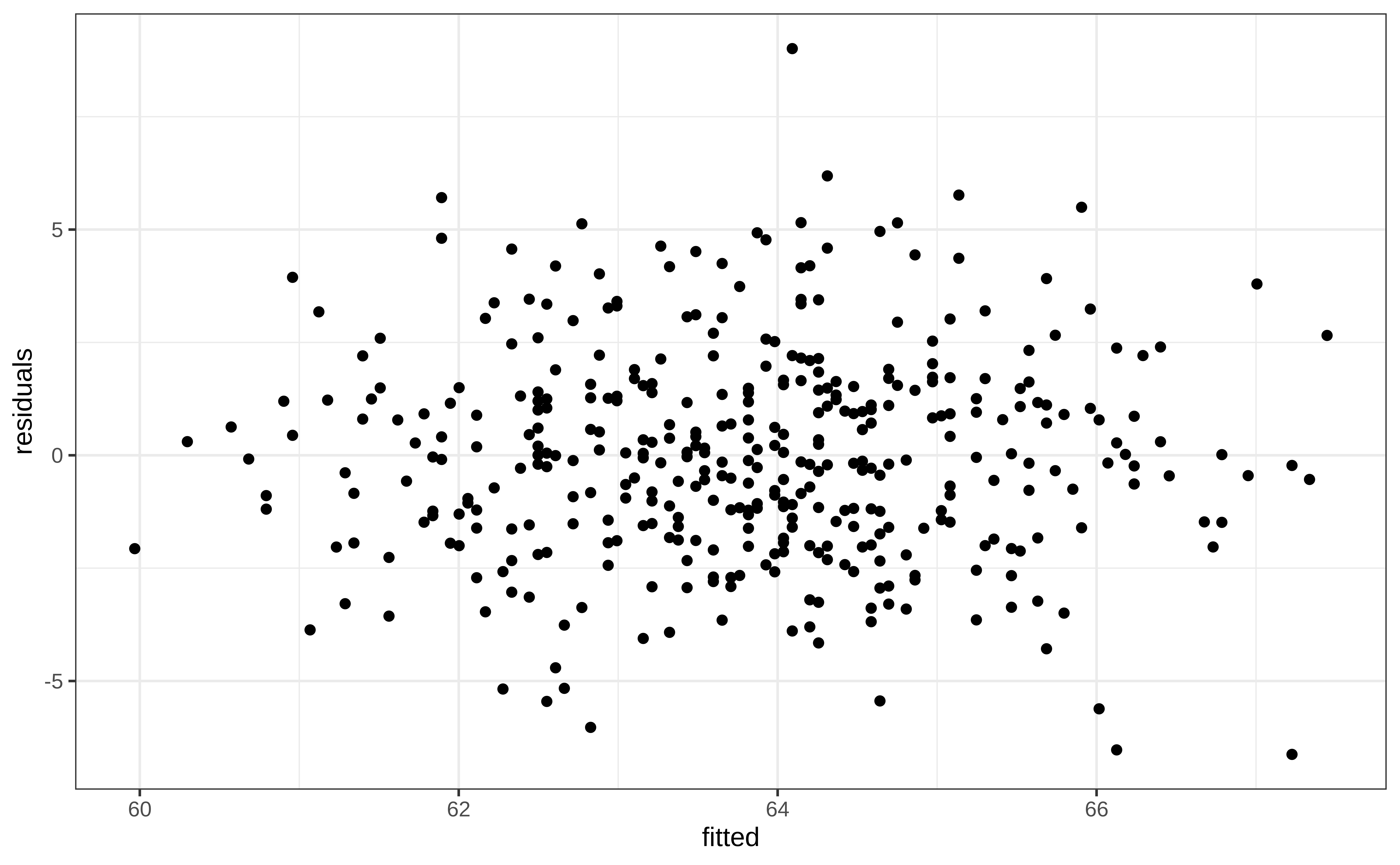
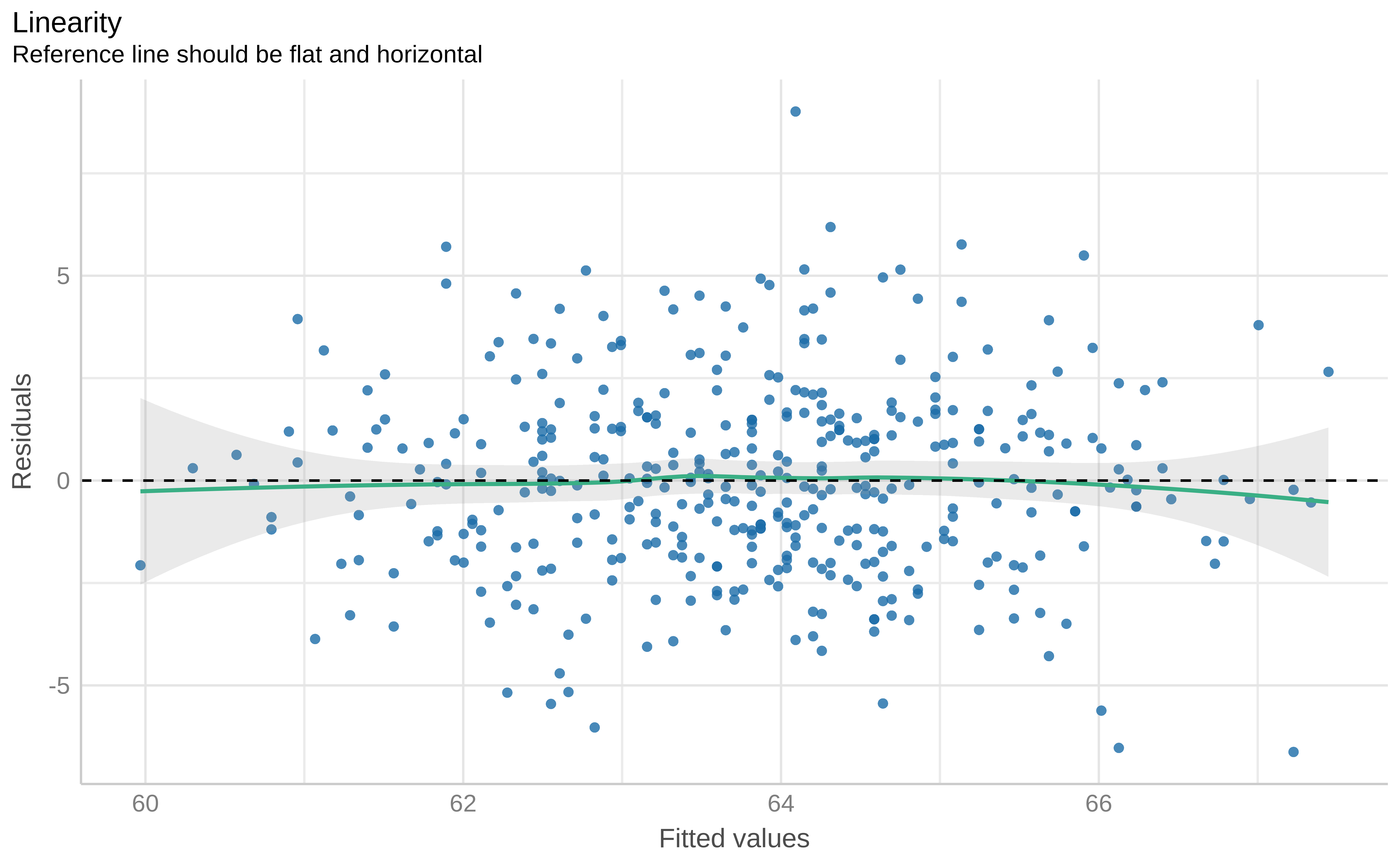
Residuals vs fitted (1/3)
Rows: 400
Columns: 4
$ mother_height   <dbl> 58.8, 65.4, 65.5, 63.2, 60.1, 61.2, 60.8, 63.7, 63.8, …
$ daughter_height <dbl> 62.7, 66.2, 62.8, 62.2, 65.1, 64.8, 63.4, 64.3, 62.5, …
$ fitted          <dbl> 61.78260, 65.41120, 65.46618, 64.20167, 62.49733, 63.1…
$ residuals       <dbl> 0.9173961, 0.7887997, -2.6661790, -2.0016682, 2.602672…
Residuals vs fitted (2/3)
Residuals vs fitted (3/3)
Takeaways
Takeaway
- Simple linear regression
- OLS
- Slope and Intercept (interpretation)
- Fitted values
- Residuals
- Residuals vs Fitted
- fitting regression:
fit() - regression summary:
summary(),tidy(),glance(),parameters(),performance(),check_model(),fitted(),residuals(),resid() - packages:
broom,parametersandperformance
Homework
Create an R Script out of the R code in the presentation.
References
References
