library(tidyverse)       # for data wrangling
library(alr4)            # for the data sets #
library(GGally)
library(parameters)
library(performance)
library(see)
library(car)
library(broom)
library(modelsummary)
library(texreg)

ggplot2::theme_set(ggplot2::theme_bw())

knitr::opts_chunk$set(
  fig.width = 10,
  fig.asp = 0.5,
  fig.retina = 3,
  dpi = 300,
  out.width = "100%",
  message = FALSE,
  echo = TRUE,
  cache = TRUE
)


my_gof <- function(fit_obj, digits = 4) {
  sum_fit <- summary(fit_obj)

  stars <-
    pf(sum_fit$fstatistic[1],
       sum_fit$fstatistic[2],
       sum_fit$fstatistic[3],
       lower.tail=FALSE) %>%
    symnum(corr = FALSE, na = FALSE,
           cutpoints = c(0,  .001,.01,.05,  1),
           symbols   =  c("***","**","*"," ")) %>%
    as.character()

  list(
    # `R^2` = sum_fit$r.squared %>% round(digits),
    # `Adj. R^2` = sum_fit$adj.r.squared %>% round(digits),
    # `Num. obs.` = sum_fit$residuals %>% length(),
    `Num. df` = sum_fit$df[[2]],
    `F statistic` =
      str_c(sum_fit$fstatistic[1] %>% round(digits), " ", stars)
  )
}

screen_many_regs <-
  function(fit_obj_list, ..., digits = 4, single.row = TRUE) {

    if (class(fit_obj_list) == "lm")
      fit_obj_list <- list(fit_obj_list)

    if (length(rlang::dots_list(...)) > 0)
      fit_obj_list <- fit_obj_list %>% append(rlang::dots_list(...))

    # browser()
    fit_obj_list %>%
      screenreg(
        custom.note =
          map2_chr(., seq_along(.), ~ {
            str_c("Model ", .y, " ", as.character(.x$call)[[2]])
          }) %>%
          c("*** p < 0.001; ** p < 0.01; * p < 0.05", .) %>%
          str_c(collapse = "\n") ,
        digits = digits,
        single.row = single.row,
        custom.gof.rows =
          map(., ~my_gof(.x, digits)) %>%
          transpose() %>%
          map(unlist),
        reorder.gof = c(3, 4, 5, 1, 2)
      )
}Hedonic model
MP223 - Applied Econometrics Methods for the Social Sciences
Eduard Bukin
R setup
Problem Setting
We would like to assess the effect of the “Conservation Reserve Program” (CPR) on the agricultural land prices in Minnesota in 2002-2011.
Conservation Reserve Program
is a subsidy
obligates farms NOT TO GROW ANY CROPS on the enrolled land
pays monetary compensation in exchange;
As this is a risk less income, it may increase the land price.
However, if the land is productive, such set-aside measure may reduce farmland price.
Hedonic Model overview
Hedonic prices is an econometric approach of quantifying monetary values of differentiated characteristics of goods and services, which are subjects of economic exchange.
For example, agricultural land.
- It has such characteristics as: location, slope, environmental limitation, farmers’ accessibility, climate, expected rainfall, soil salinity, nutrient content, irrigation availability and other.
Hedonic Theory (1/2)
According to (Palmquist 1989), hedonic model of agricultural land price is based on the equilibrium between Offer and Bid functions. Author uses partial equilibrium approach to prove this.
\[\phi(\hat{z}, \tilde{z}, \pi^{S^{'}}, r, \beta) = R = \pi^{S^{'}} + C(\hat{z}, \tilde{z}, r, \beta)\]
\(R(\cdot)\) - realized land price (rental of sales);
\(\hat{z}\) - land characteristics exogenous to land owner;
\(\tilde{z}\) - land characteristics in control of land owner;
\(r\) - inputs prices;
\(\beta\) - technologies and opportunities such as credit availability;
\(\pi^{S^{'}}\) - expected profit of agricultural producers from land;
Hedonic Theory (2/2)
Essentially, causal function of the land rental price could be written as:
\[R = R(\hat{z}, \tilde{z}, \pi^{S^{'}}, r, \beta)\]
Important
This is a causal relationship because (Palmquist 1989) provides solid theoretical justification for it.
What are the differentiated land characteristics?
Affected by land owner:
- a.
- b.
- c.
Not affected by land owner:
- a.
- b.
- c.
Data
Data set MinnLand from (Taff and Weisberg 2007).
acrePrice- sale price in dollars per acre;acres- size of the farm in acres;region- region in the state Minnesota;year- year of the land sales translation;crpPct- the percentage of all farm acres enrolled in CRP;tillable- percentage of farm acreage that is rated arable by the assessor;productivity- average agronomic productivity scaled 1 to 100, with larger numbers for more productive land;
Loading data
Code
Rows: 18,700
Columns: 7
$ acrePrice    <dbl> 766, 733, 850, 975, 886, 992, 623, 1382, 855, 364, 807, 4…
$ acres        <int> 82, 30, 150, 160, 90, 120, 170, 100, 120, 160, 158, 83, 1…
$ region       <fct> Northwest, Northwest, Northwest, Northwest, Northwest, No…
$ year         <dbl> 2002, 2003, 2002, 2003, 2002, 2003, 2003, 2003, 2003, 200…
$ tillable     <dbl> 94, 63, 47, 86, NA, 83, 42, 35, 46, 10, 29, 36, 14, 71, 9…
$ crpPct       <dbl> 0, 0, 0, 0, 0, 0, 0, 0, 0, 0, 0, 0, 0, 0, 0, 0, 0, 0, 0, …
$ productivity <int> NA, NA, NA, NA, NA, NA, NA, NA, NA, NA, NA, NA, NA, NA, N…
Summary statistics (1/2)
Code
dta %>%
  mutate(id = row_number()) %>%
  pivot_longer(
    cols = c(acrePrice, acres, year, tillable, crpPct, productivity),
    names_to = "var",
    values_to = "val"
  ) %>%
  group_by(var) %>%
  summarise(across(
    c(val),
    list(
      mean = ~ mean(.x, na.rm = TRUE),
      sd = ~ sd(.x, na.rm = TRUE),
      meadian = ~ median(.x, na.rm = TRUE),
      n_miss = ~ sum(is.na(.x), na.rm = TRUE),
      min = ~ min(.x, na.rm = TRUE),
      max = ~ max(.x, na.rm = TRUE)
    )
  ),
  n = n())
# A tibble: 6 × 8
var val_mean val_sd val_meadian val_n_miss val_min val_max n
<chr> <dbl> <dbl> <dbl> <int> <dbl> <dbl> <int>
1 acrePrice 2787. 1914. 2442 0 108 15000 18700
2 acres 113. 128. 80 0 1 6970 18700
3 crpPct 4.16 17.2 0 0 0 100 18700
4 productivity 66.6 13.5 68 9717 1 99 18700
5 tillable 80.7 22.8 92 1212 0 100 18700
6 year 2006. 2.51 2006 0 2002 2011 18700Summary statistics (2/2)
               Unique (#) Missing (%)   Mean     SD    Min Median     Max
1    acrePrice       5696           0 2787.3 1914.0  108.0 2442.0 15000.0
2        acres        596           0  112.7  128.5    1.0   80.0  6970.0
3         year         10           0 2006.4    2.5 2002.0 2006.0  2011.0
4     tillable        102           6   80.7   22.8    0.0   92.0   100.0
5       crpPct        101           0    4.2   17.2    0.0    0.0   100.0
6 productivity         96          52   66.6   13.5    1.0   68.0    99.0
Visual inspection: scatter plots
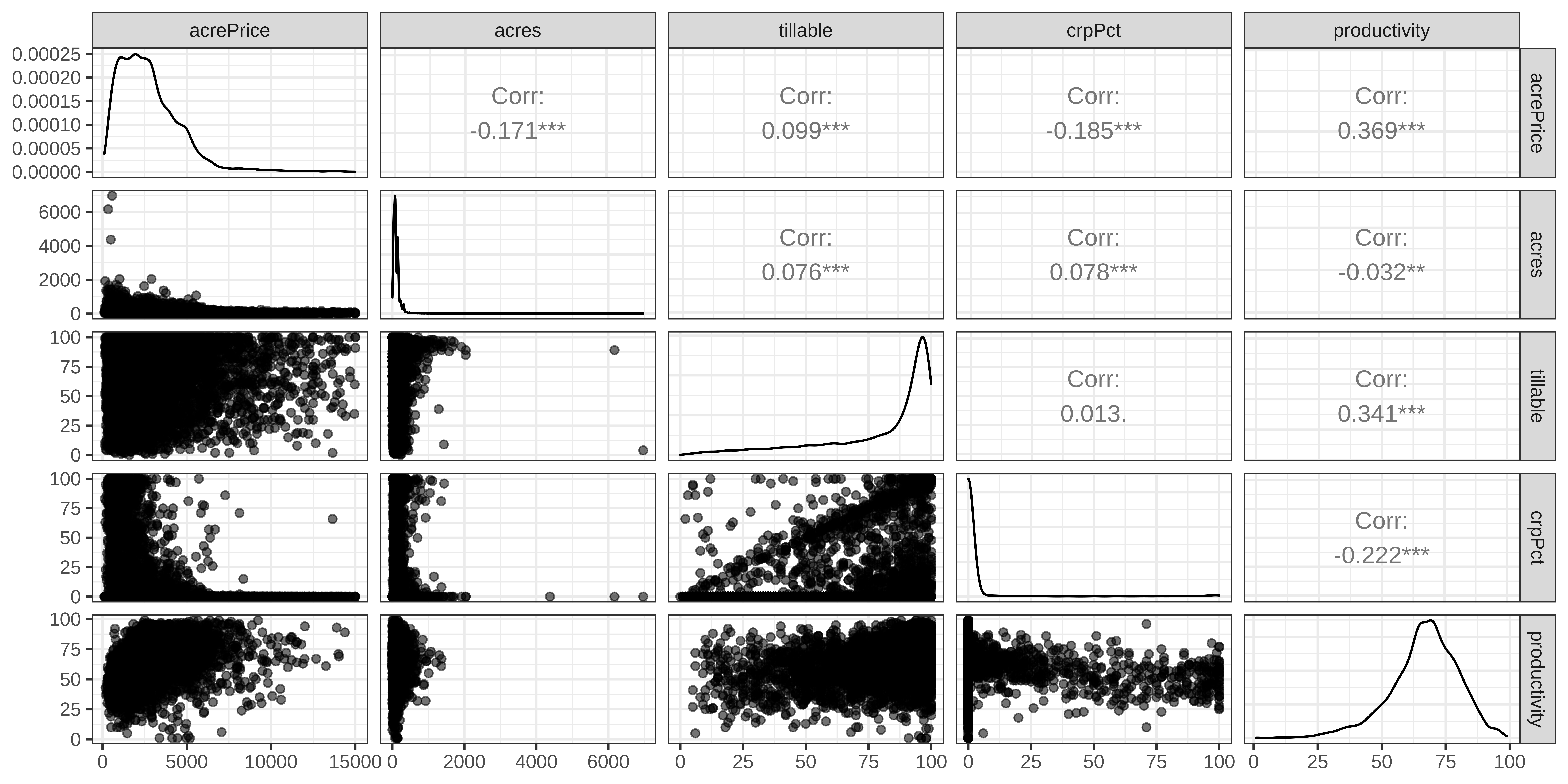
Hedonic Regression
Regression. Summary
Code
Call:
lm(formula = acrePrice ~ crpPct + acres + region + year + tillable +
    productivity, data = dta)

Residuals:
    Min      1Q  Median      3Q     Max
-3663.2  -572.0  -132.8   356.3 11029.3

Coefficients:
                      Estimate Std. Error t value Pr(>|t|)
(Intercept)         -6.476e+05  9.554e+03 -67.781   <2e-16 ***
crpPct              -8.288e+00  8.693e-01  -9.534   <2e-16 ***
acres               -1.166e+00  1.337e-01  -8.720   <2e-16 ***
regionWest Central   9.474e+02  4.703e+01  20.145   <2e-16 ***
regionCentral        1.798e+03  5.234e+01  34.357   <2e-16 ***
regionSouth West     1.257e+03  4.727e+01  26.595   <2e-16 ***
regionSouth Central  1.669e+03  5.070e+01  32.923   <2e-16 ***
regionSouth East     1.939e+03  5.875e+01  33.002   <2e-16 ***
year                 3.230e+02  4.764e+00  67.792   <2e-16 ***
tillable            -2.502e+00  7.881e-01  -3.175   0.0015 **
productivity         2.445e+01  1.078e+00  22.686   <2e-16 ***
---
Signif. codes:  0 '***' 0.001 '**' 0.01 '*' 0.05 '.' 0.1 ' ' 1

Residual standard error: 1079 on 8776 degrees of freedom
  (9913 observations deleted due to missingness)
Multiple R-squared:  0.5179,    Adjusted R-squared:  0.5174
F-statistic: 942.8 on 10 and 8776 DF,  p-value: < 2.2e-16
Regression. Interpretation of the coefficients
Parameter              | Coefficient |      SE |                   95% CI | t(8776) |      p
--------------------------------------------------------------------------------------------
(Intercept)            |   -6.48e+05 | 9553.71 | [ -6.66e+05,  -6.29e+05] |  -67.78 | < .001
crpPct                 |       -8.29 |    0.87 | [     -9.99,      -6.58] |   -9.53 | < .001
acres                  |       -1.17 |    0.13 | [     -1.43,      -0.90] |   -8.72 | < .001
region [West Central]  |      947.38 |   47.03 | [    855.19,    1039.56] |   20.15 | < .001
region [Central]       |     1798.21 |   52.34 | [   1695.61,    1900.81] |   34.36 | < .001
region [South West]    |     1257.17 |   47.27 | [   1164.51,    1349.83] |   26.60 | < .001
region [South Central] |     1669.12 |   50.70 | [   1569.74,    1768.50] |   32.92 | < .001
region [South East]    |     1938.87 |   58.75 | [   1823.71,    2054.04] |   33.00 | < .001
year                   |      322.97 |    4.76 | [    313.63,     332.30] |   67.79 | < .001
tillable               |       -2.50 |    0.79 | [     -4.05,      -0.96] |   -3.18 | 0.002
productivity           |       24.45 |    1.08 | [     22.33,      26.56] |   22.69 | < .001
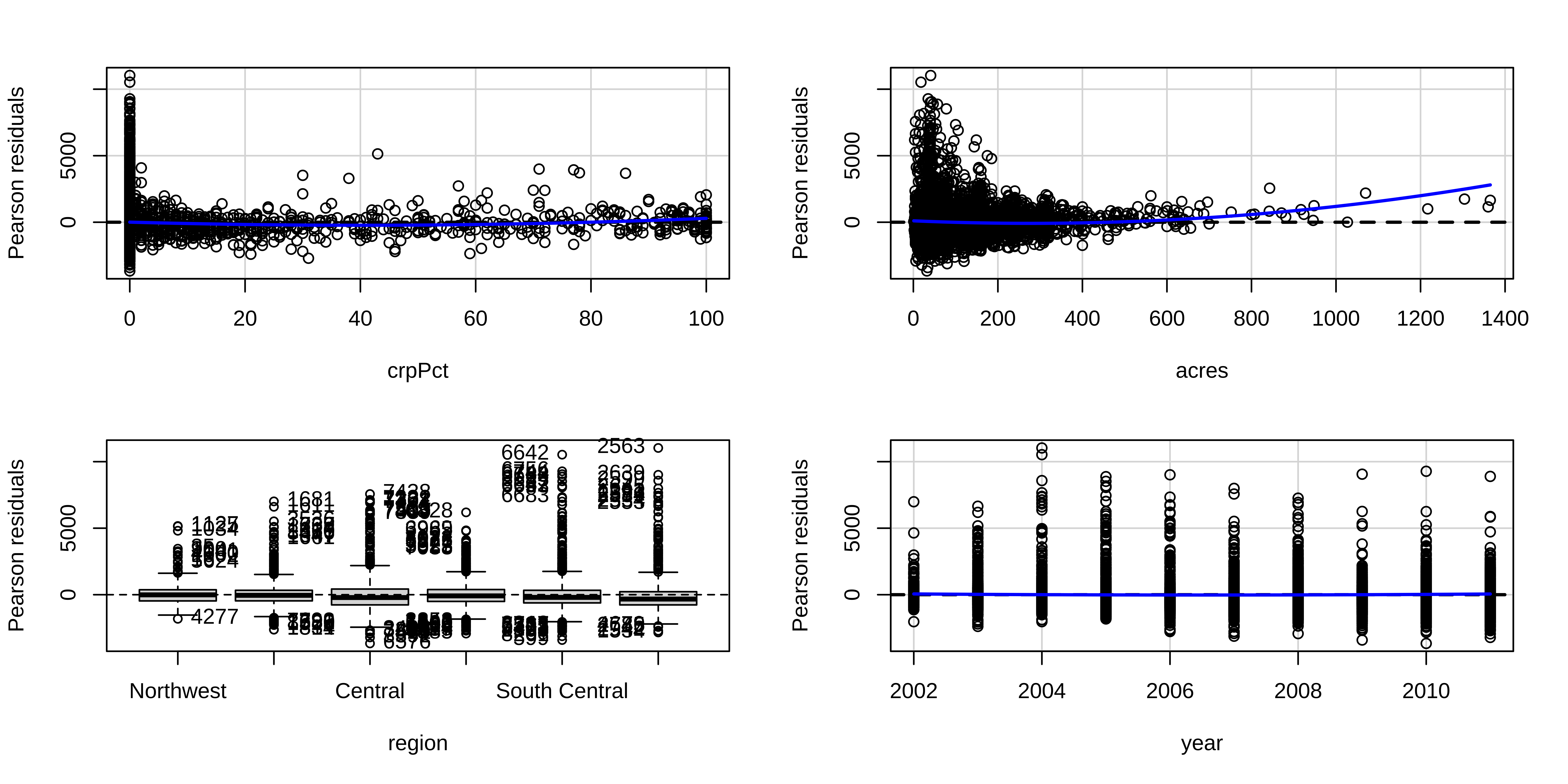
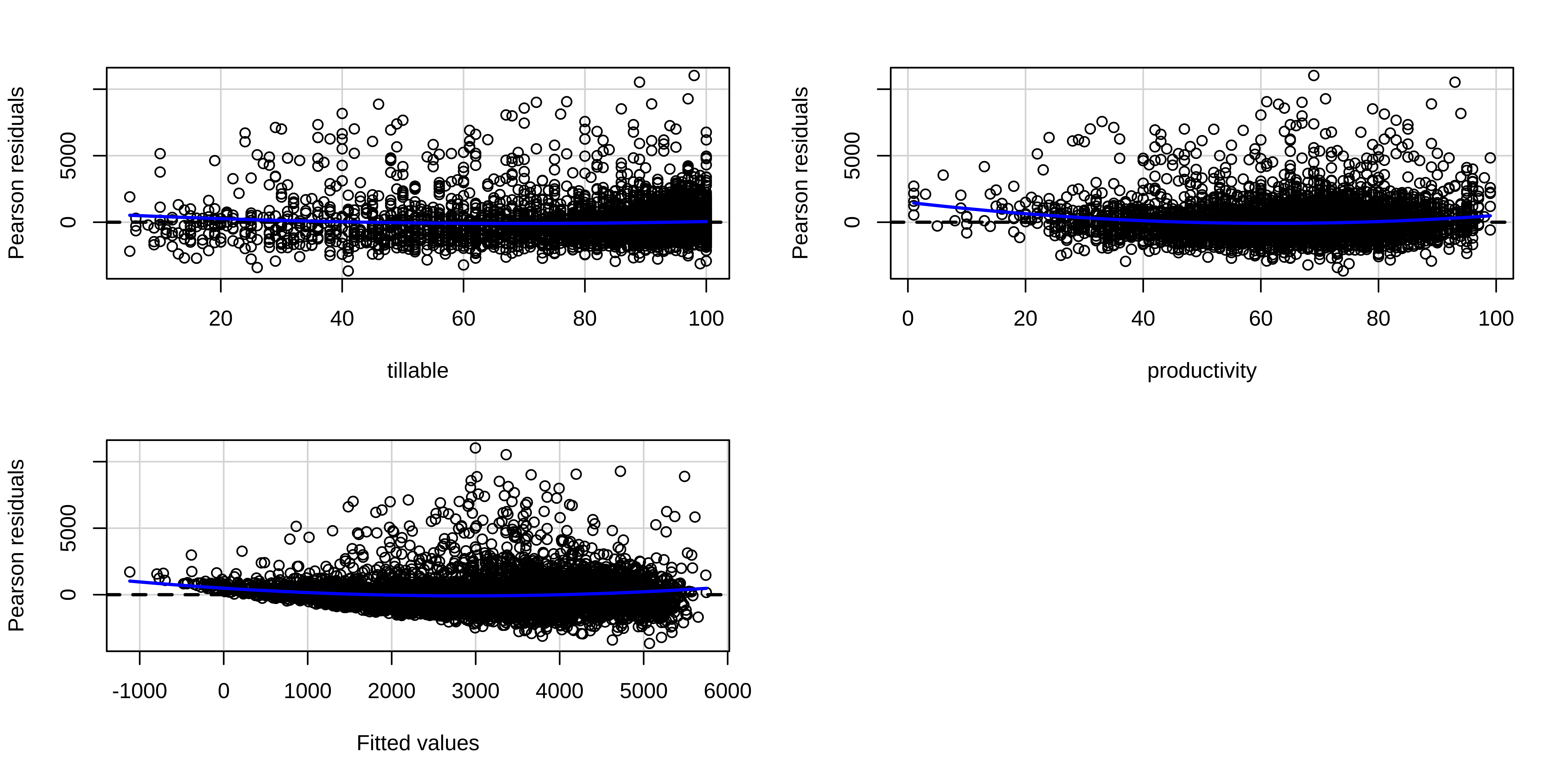
Checking Linearity 1/3
Checking Linearity 2/3
             Test stat Pr(>|Test stat|)
crpPct          3.8991        9.727e-05 ***
acres           7.0230        2.334e-12 ***
region
year            2.0206          0.04335 *
tillable        4.9822        6.407e-07 ***
productivity   11.1526        < 2.2e-16 ***
Tukey test     11.0991        < 2.2e-16 ***
---
Signif. codes:  0 '***' 0.001 '**' 0.01 '*' 0.05 '.' 0.1 ' ' 1
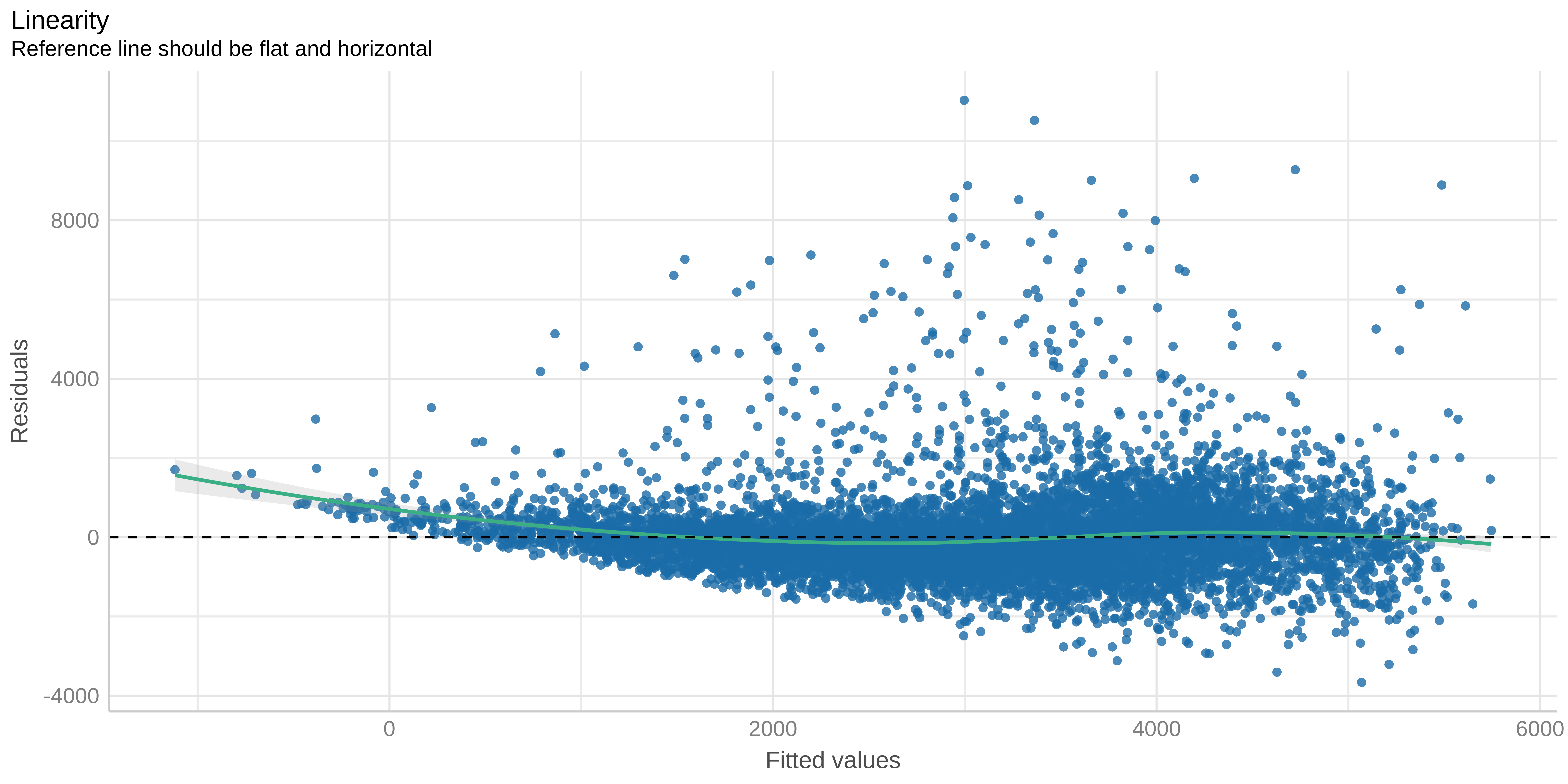
Checking Linearity 3/3
Takeaways
Takeaway
- Multiple linear regression
- Hedonic model
- Slope and Intercept (interpretation)
- Residuals vs Fitted
Homework
Create an R Script out of the R code in the presentation.
References
References
