AE06-01 linear transformation and interaction term: the toolbox

Setup

library(tidyverse)
library(alr4)
library(GGally)
library(parameters)
library(performance)
library(see)
library(car)
library(broom)
library(modelsummary)
library(texreg)
library(correlation)
library(patchwork)
library(lmtest)
library(sandwich)
library(clubSandwich)
library(forcats)
library(modelbased)
library(emmeans)
library(ggeffects)

knitr::opts_chunk$set(
  fig.align = "center",
  fig.width = 16,
  fig.asp = 0.618,
  fig.retina = 1,
  out.width = "100%", 
  message = FALSE,
  warning = FALSE,
  echo = TRUE
)

Goals:

• Learn what is the interaction term in regression and how to use it;

Exercise 1. Interaction with a dummy variable

1.1 Load data, compute, select, filter

• total amount of parents education paredu as a sum of years of their education

dta <- 
  wooldridge::wage1 %>% 
  as_tibble() %>% 
  mutate(sex = ifelse(female == 0, "male", "female") %>% 
           as_factor() %>% 
           fct_rev()) %>%
  select(wage, educ, exper, sex)

Variables are:

• wage: average hourly earnings
• educ: years of education
• exper: years potential experience
• sex: sex of the respondents

1.2 Built pairs plot and descriptive statistics

library(GGally)
ggpairs(dta, aes(group = sex, colour = sex, alpha = 0.3))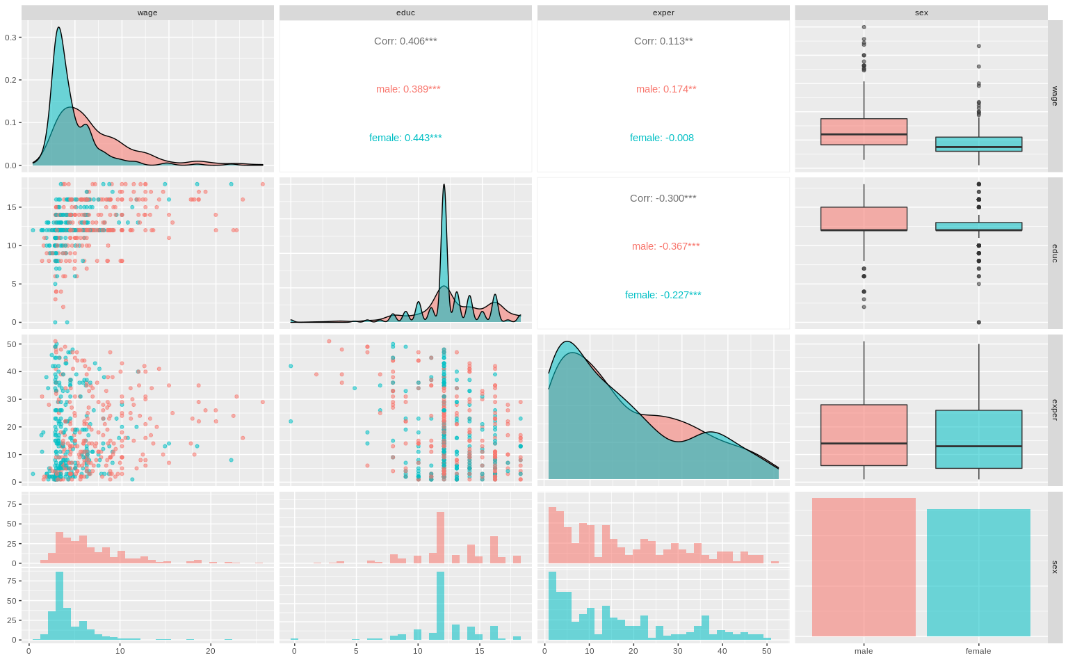

library(modelsummary)
dta %>% datasummary_skim()

	Unique (#)	Missing (%)	Mean	SD	Min	Median	Max
wage	241	0	5.9	3.7	0.5	4.7	25.0
educ	18	0	12.6	2.8	0.0	12.0	18.0
exper	51	0	17.0	13.6	1.0	13.5	51.0

1.3 Regression without interaction terms

fit_1 <- lm(wage ~ educ + exper + sex, data = dta)
parameters(fit_1)

Parameter    | Coefficient |   SE |         95% CI | t(522) |      p
--------------------------------------------------------------------
(Intercept)  |       -1.73 | 0.75 | [-3.21, -0.25] |  -2.30 | 0.022 
educ         |        0.60 | 0.05 | [ 0.50,  0.70] |  11.79 | < .001
exper        |        0.06 | 0.01 | [ 0.04,  0.08] |   6.18 | < .001
sex [female] |       -2.16 | 0.27 | [-2.69, -1.62] |  -7.97 | < .001

performance(fit_1)

# Indices of model performance

AIC      |      BIC |    R2 | R2 (adj.) |  RMSE | Sigma
-------------------------------------------------------
2681.472 | 2702.798 | 0.309 |     0.305 | 3.066 | 3.078

Diagnostics

check_model(fit_1, check = c("linearity", "homogeneity"))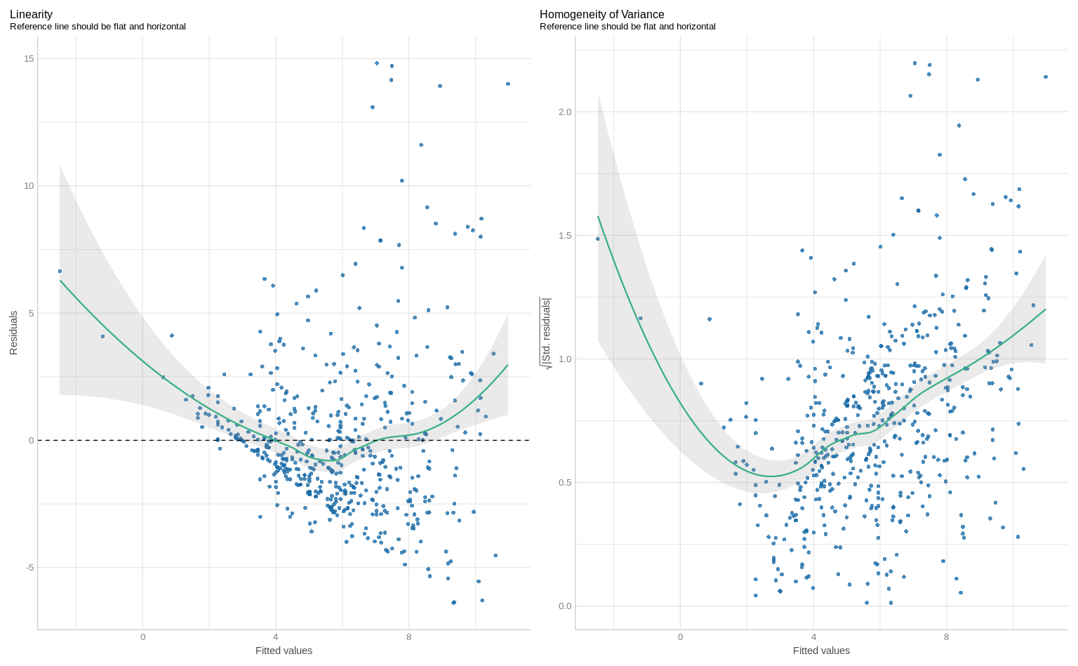

1.4 Attempting to resolve linearity

• Introduce squared education and experience terms.

# fit_2 <- lm(log(wage) ~ educ + ______ + exper + ______ + sex, 
#             data = dta)
# parameters(fit_2)
# performance(fit_2)
# check_model(fit_2, check = c("linearity", "homogeneity"))

1.5 Computing fitted values

Calculate fitted values based on the regressionfit_2 for:

• a women and men;
• with 10 and 11 years of experience;
• 10, 11, 16 and 17 years of education;

Built a tibble() with the covariates for prediction:

# pred_dta_1 <-
#   tibble(
#     sex = ______,
#     ______ = c(10, 11, ______, 10, 11, 16, 17),
#     exper = ______
#   ) %>%
#   bind_rows(mutate(., sex = "male"))

Predict fitted values and write them to the variable fitted

# ______(______, pred_dta_1)
# 
# pred_dta_2 <- 
#   pred_dta_1 %>% 
#   mutate(fitted_values = ______(______, pred_dta_1))

Compute predicted salary and save it into the variable pred_wage;

# pred_dta_3 <- 
#   pred_dta_2 %>% 
#   mutate(pred_wage = ______(fitted_values))
# pred_dta_3

1.6 Computing slope for squared term

The slope depends on the value of regressor

\(\frac{\partial \text{ wage}}{\partial \text{ educ}} = -0.0306529 + 2 \times 0.0048716 \times \text{educ}\)

What is the effect of an additional year of education on wage, given that current level of education is 10 or 16 years?

• Estimate slopes manually and using modelbased;
• Interpret the results;
• Plot the slope;
• What is the meaning of the shaded area?

library(modelbased)
library(emmeans)

## Estimate slope of educ for 10 and 11 years of education, manually
# parameters(fit_2)
# ______ + ______ * ______ * ______
# ______ + ______ * ______ * ______

# # Estimating slopes manually for our data
# pred_dta_3 %>% 
#   select(- pred_wage  ) %>%
#   pivot_wider(names_from = educ, values_from = fitted_values) %>% 
#   mutate(beta_educ_10_11 = `11`-`10`,
#          beta_educ_16_17 = `17`-`16`)

# # Using function estimate_slopes
# estimate_slopes(fit_2, trend = "educ")
# 
# # add `at = "educ"`
# estimate_slopes(fit_2, trend = ______, at = "educ")
# 
# # Add `at = list(educ = c(10, 11))`
# estimate_slopes(fit_2, trend = ______, at = list(educ = c(10, 11)))
# 
# # adding plot
# estimate_slopes(fit_2, trend = ______, at = ______) %>% plot()
# 
# # adding plot at sex and education
# estimate_slopes(fit_2, trend = ______, at = c("educ", "sex")) %>% ______()

Marginal effects to report

1.7 Predicted values given linear transformation

library(ggeffects)

# pred_dta_3
# 
# # using ggpredict
# ggpredict(fit_2, terms = "educ")
# 
# # back.transform = F
# ggpredict(fit_2, ______ = "educ", back.transform = F)
# 
# # `terms = c("educ", "sex")`
# ggpredict(fit_2, terms = c("educ", "sex"), ______)
# 
# # Plotting
# ggpredict(fit_2, ______ = "educ", back.transform = F) %>% plot()
# ggpredict(fit_2, ______) %>% plot()
# ggpredict(fit_2, terms = c(______)) %>% plot()

1.8 Effect of a dummy variable

In the regression coefficients, sex variable has a coefficient of -0.32

# ggpredict(fit_2, ______ = "sex") %>% plot()
# ggpredict(fit_2, ______ = "sex", back.transform = F)
# parameters(fit_2)

Exercise 2. Interaction term

2.1 Adding an interaction term between sex and education

# fit_3 <- lm(log(wage) ~ 
#               educ + I(educ ^ 2) + exper + I(exper ^ 2) + sex + 
#               ______, 
#             data = dta)
# parameters(fit_3)
# performance(fit_3)
# check_model(fit_3, check = c("linearity", "homogeneity"))

2.2 Interpreting the interaction term

Interpreting the changing slopes

# estimate_slopes(______, ______ = "educ", at = "educ") %>% plot()
# estimate_slopes(______, ______ = "educ", ______ = c("sex", "educ")) %>% plot()
# estimate_slopes(______, ______ = "educ", ______ = c("sex")) %>% plot()

Interpreting the fitted values

# ggpredict(______, ______ = "educ") %>% plot()
# ggpredict(______, ______ = c("sex", "educ")) %>% plot()
# ggpredict(______, ______ = c("educ", "sex")) %>% plot()
# ggpredict(______, ______ = c("educ", "sex")) %>% plot(add.data = TRUE)

Solutions

Code

dta <- 
  wooldridge::wage1 %>% 
  as_tibble() %>% 
  mutate(sex = ifelse(female == 0, "male", "female") %>% 
           as_factor() %>% 
           fct_rev(),
         lwage = log(wage)) %>%
  select(lwage, wage, educ, exper, sex)

# 1.2 Built pairs plot and descriptive statistics
library(GGally)
ggpairs(dta, aes(group = sex, colour = sex, alpha = 0.3))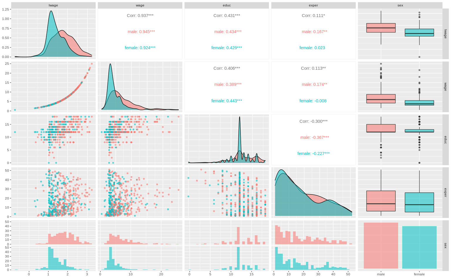

Code

library(modelsummary)
dta %>% datasummary_skim()

	Unique (#)	Missing (%)	Mean	SD	Min	Median	Max
lwage	241	0	1.6	0.5	−0.6	1.5	3.2
wage	241	0	5.9	3.7	0.5	4.7	25.0
educ	18	0	12.6	2.8	0.0	12.0	18.0
exper	51	0	17.0	13.6	1.0	13.5	51.0

Code

# 1.3 Regression without interaction terms
fit_1 <- lm(wage ~ educ + exper + sex, data = dta)
parameters(fit_1)

Parameter    | Coefficient |   SE |         95% CI | t(522) |      p
--------------------------------------------------------------------
(Intercept)  |       -1.73 | 0.75 | [-3.21, -0.25] |  -2.30 | 0.022 
educ         |        0.60 | 0.05 | [ 0.50,  0.70] |  11.79 | < .001
exper        |        0.06 | 0.01 | [ 0.04,  0.08] |   6.18 | < .001
sex [female] |       -2.16 | 0.27 | [-2.69, -1.62] |  -7.97 | < .001

Code

performance(fit_1)

# Indices of model performance

AIC      |      BIC |    R2 | R2 (adj.) |  RMSE | Sigma
-------------------------------------------------------
2681.472 | 2702.798 | 0.309 |     0.305 | 3.066 | 3.078

Code

check_model(fit_1, check = c("linearity", "homogeneity"))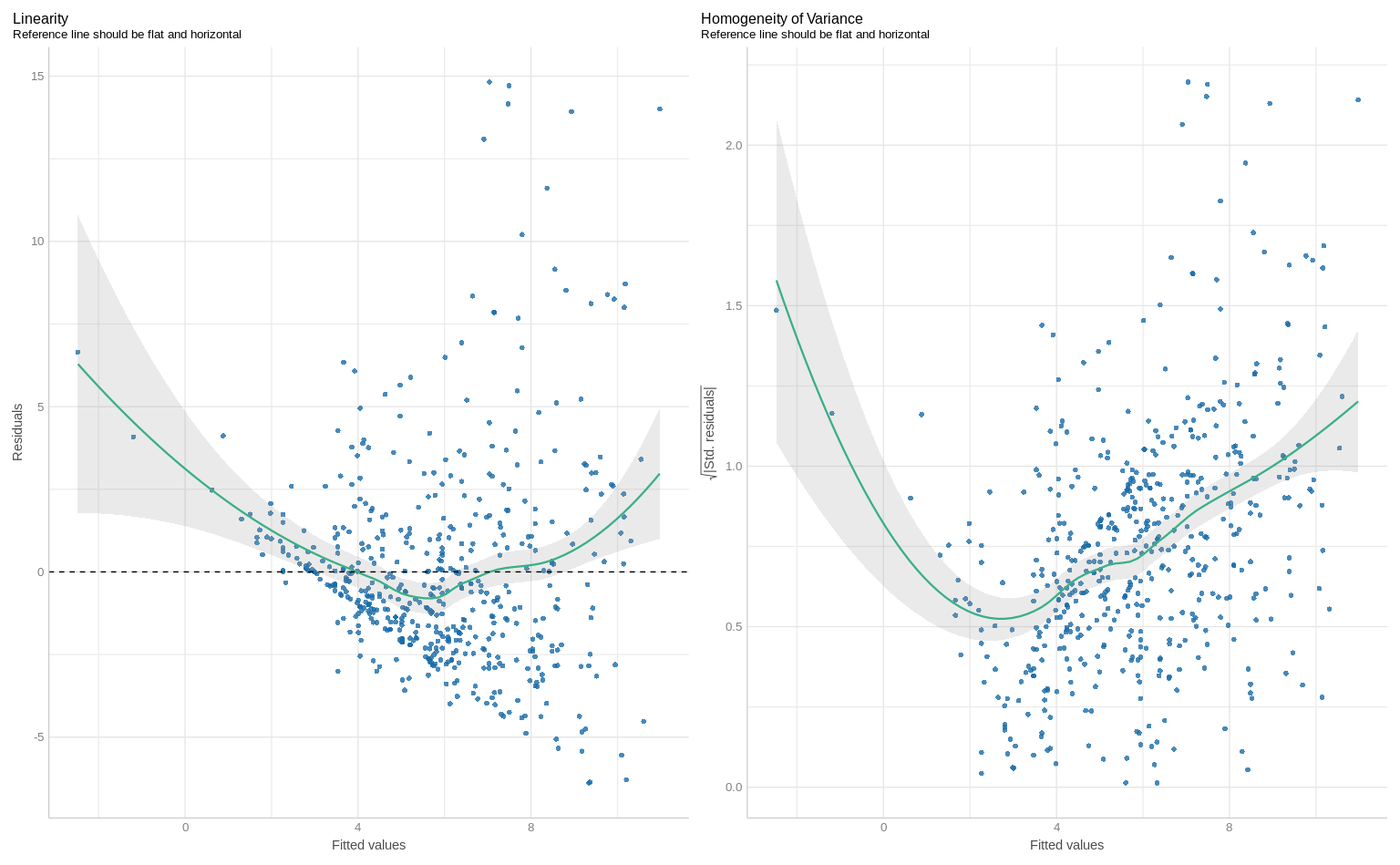

Code

# 1.4 Attempting to resolve linearity
fit_2 <- lm(log(wage) ~ educ + I(educ ^ 2) + exper + I(exper ^ 2) + sex, 
            data = dta)
parameters(fit_2)

Parameter    | Coefficient |       SE |         95% CI | t(520) |      p
------------------------------------------------------------------------
(Intercept)  |        1.02 |     0.19 | [ 0.64,  1.39] |   5.32 | < .001
educ         |       -0.03 |     0.03 | [-0.09,  0.03] |  -1.00 | 0.316 
educ^2       |    4.87e-03 | 1.26e-03 | [ 0.00,  0.01] |   3.86 | < .001
exper        |        0.04 | 4.77e-03 | [ 0.03,  0.05] |   8.37 | < .001
exper^2      |   -7.19e-04 | 1.06e-04 | [ 0.00,  0.00] |  -6.76 | < .001
sex [female] |       -0.32 |     0.04 | [-0.39, -0.25] |  -8.84 | < .001

Code

performance(fit_2)

# Indices of model performance

AIC      |      BIC |    R2 | R2 (adj.) |  RMSE | Sigma
-------------------------------------------------------
2265.351 | 4002.887 | 0.416 |     0.411 | 0.406 | 0.408

Code

check_model(fit_2, check = c("linearity", "homogeneity"))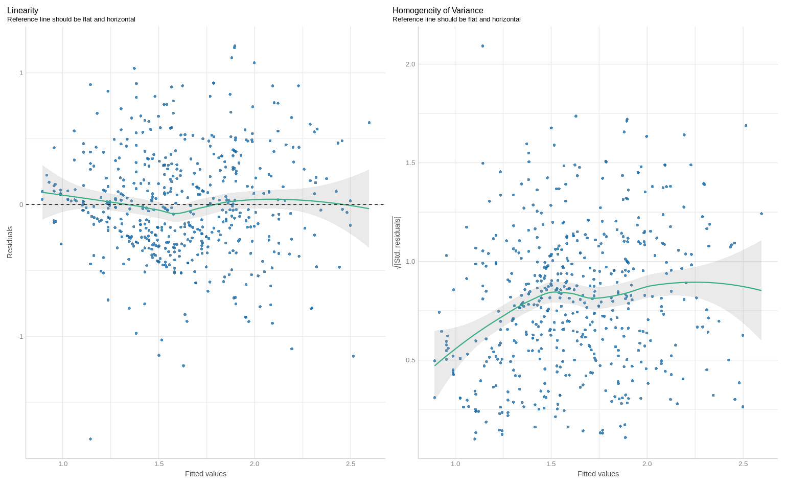

Code

# 1.5 Computing fitted values
pred_dta_1 <-
  tibble(
    sex = "female",
    educ = c(10, 11, 16, 17, 10, 11, 16, 17),
    exper = c(10, 10, 10, 10, 11, 11, 11, 11)
  ) %>%
  bind_rows(mutate(., sex = "male"))

# Predict fitted values and write them to the variable fitted
pred_dta_2 <- 
  pred_dta_1 %>% 
  mutate(fitted_values = predict(fit_2, pred_dta_1))


# Compute predicted salary and save it into the variable `pred_wage`;
pred_dta_3 <- 
  pred_dta_2 %>% 
  mutate(pred_wage = exp(fitted_values))
pred_dta_3

# A tibble: 16 × 5
   sex     educ exper fitted_values pred_wage
   <chr>  <dbl> <dbl>         <dbl>     <dbl>
 1 female    10    10          1.21      3.34
 2 female    11    10          1.28      3.58
 3 female    16    10          1.78      5.94
 4 female    17    10          1.91      6.76
 5 female    10    11          1.23      3.42
 6 female    11    11          1.30      3.67
 7 female    16    11          1.81      6.09
 8 female    17    11          1.94      6.93
 9 male      10    10          1.52      4.59
10 male      11    10          1.60      4.93
11 male      16    10          2.10      8.17
12 male      17    10          2.23      9.31
13 male      10    11          1.55      4.71
14 male      11    11          1.62      5.06
15 male      16    11          2.13      8.38
16 male      17    11          2.26      9.54

Code

# 1.6 Computing slope for squared term
library(modelbased)
library(emmeans)

# Estimate slope of educ for 10 and 11 years of education, manually
-0.0306529 + 0.0048716 * 2 * 10

[1] 0.0667791

Code

-0.0306529 + 0.0048716 * 2 * 11

[1] 0.0765223

Code

# Estimating slopes manually for our data
pred_dta_3 %>% 
  # filter(educ %in% c(10, 11)) %>% 
  select(- pred_wage  ) %>%
  pivot_wider(names_from = educ, values_from = fitted_values) %>% 
  mutate(beta_educ_10_11 = `11`-`10`,
         beta_educ_16_17 = `17`-`16`)

# A tibble: 4 × 8
  sex    exper  `10`  `11`  `16`  `17` beta_educ_10_11 beta_educ_16_17
  <chr>  <dbl> <dbl> <dbl> <dbl> <dbl>           <dbl>           <dbl>
1 female    10  1.21  1.28  1.78  1.91          0.0717           0.130
2 female    11  1.23  1.30  1.81  1.94          0.0717           0.130
3 male      10  1.52  1.60  2.10  2.23          0.0717           0.130
4 male      11  1.55  1.62  2.13  2.26          0.0717           0.130

Code

# Using function estimate_slopes
estimate_slopes(fit_2, trend = "educ")

Estimated Marginal Effects

Coefficient |       SE |       95% CI | t(520) |      p
-------------------------------------------------------
0.09        | 7.15e-03 | [0.08, 0.11] |  12.85 | < .001
Marginal effects estimated for educ

Code

# add `at = "educ"`
estimate_slopes(fit_2, trend = "educ", at = "educ")

Estimated Marginal Effects

educ  | Coefficient |       SE |        95% CI | t(520) |      p
----------------------------------------------------------------
0.00  |       -0.03 |     0.03 | [-0.09, 0.03] |  -1.00 | 0.317 
2.00  |       -0.01 |     0.03 | [-0.06, 0.04] |  -0.43 | 0.665 
4.00  |    8.41e-03 |     0.02 | [-0.03, 0.05] |   0.40 | 0.686 
6.00  |        0.03 |     0.02 | [ 0.00, 0.06] |   1.73 | 0.084 
8.00  |        0.05 |     0.01 | [ 0.02, 0.07] |   4.04 | < .001
10.00 |        0.07 | 8.19e-03 | [ 0.05, 0.08] |   8.16 | < .001
12.00 |        0.09 | 6.89e-03 | [ 0.07, 0.10] |  12.53 | < .001
14.00 |        0.11 | 8.87e-03 | [ 0.09, 0.12] |  11.93 | < .001
16.00 |        0.13 |     0.01 | [ 0.10, 0.15] |   9.88 | < .001
18.00 |        0.14 |     0.02 | [ 0.11, 0.18] |   8.44 | < .001
Marginal effects estimated for educ

Code

# Add `at = list(educ = c(10, 11))`
estimate_slopes(fit_2, trend = "educ", at = list(educ = c(10, 11)))

Estimated Marginal Effects

educ  | Coefficient |       SE |       95% CI | t(520) |      p
---------------------------------------------------------------
10.00 |        0.07 | 8.19e-03 | [0.05, 0.08] |   8.16 | < .001
11.00 |        0.08 | 7.14e-03 | [0.06, 0.09] |  10.73 | < .001
Marginal effects estimated for educ

Code

# adding plot
estimate_slopes(fit_2, trend = "educ", at = "educ") %>% plot()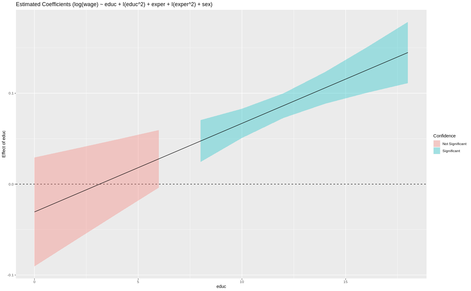

Code

# adding plot at sex and education
estimate_slopes(fit_2, trend = "educ", at = c("educ", "sex")) %>% plot()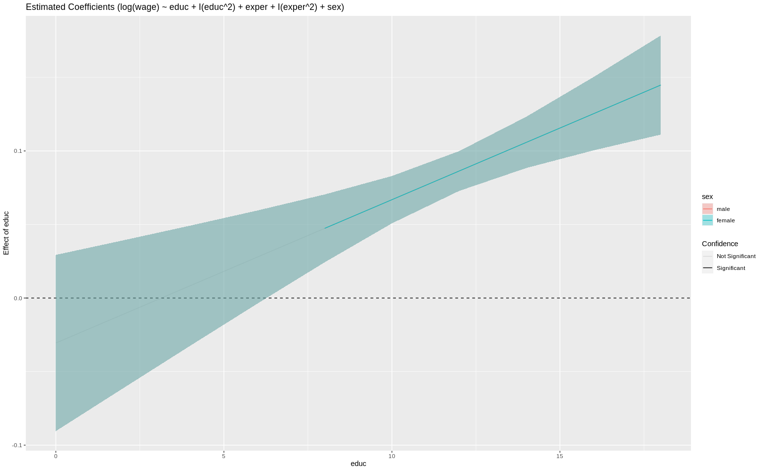

Code

# 1.7 Predicted values given linear transformation
library(ggeffects)

pred_dta_3

# A tibble: 16 × 5
   sex     educ exper fitted_values pred_wage
   <chr>  <dbl> <dbl>         <dbl>     <dbl>
 1 female    10    10          1.21      3.34
 2 female    11    10          1.28      3.58
 3 female    16    10          1.78      5.94
 4 female    17    10          1.91      6.76
 5 female    10    11          1.23      3.42
 6 female    11    11          1.30      3.67
 7 female    16    11          1.81      6.09
 8 female    17    11          1.94      6.93
 9 male      10    10          1.52      4.59
10 male      11    10          1.60      4.93
11 male      16    10          2.10      8.17
12 male      17    10          2.23      9.31
13 male      10    11          1.55      4.71
14 male      11    11          1.62      5.06
15 male      16    11          2.13      8.38
16 male      17    11          2.26      9.54

Code

# using ggpredict
ggpredict(fit_2, terms = "educ")

# Predicted values of wage

educ | Predicted |         95% CI
---------------------------------
   0 |      4.16 | [ 2.86,  6.03]
   3 |      3.96 | [ 3.16,  4.97]
   5 |      4.03 | [ 3.45,  4.71]
   7 |      4.26 | [ 3.82,  4.74]
  10 |      4.98 | [ 4.63,  5.36]
  12 |      5.80 | [ 5.45,  6.18]
  14 |      7.03 | [ 6.64,  7.45]
  18 |     11.60 | [10.37, 12.98]

Adjusted for:
* exper = 13.50
*   sex =  male

Code

# back.transform = F
ggpredict(fit_2, terms = "educ", back.transform = F)

# Predicted values of wage

educ | Predicted |       95% CI
-------------------------------
   0 |      1.42 | [1.05, 1.80]
   3 |      1.38 | [1.15, 1.60]
   5 |      1.39 | [1.24, 1.55]
   7 |      1.45 | [1.34, 1.56]
  10 |      1.61 | [1.53, 1.68]
  12 |      1.76 | [1.70, 1.82]
  14 |      1.95 | [1.89, 2.01]
  18 |      2.45 | [2.34, 2.56]

Adjusted for:
* exper = 13.50
*   sex =  male

Code

# `terms = c("educ", "sex")`
ggpredict(fit_2, terms = c("educ", "sex"), back.transform = F)

# Predicted values of wage

# sex = male

educ | Predicted |       95% CI
-------------------------------
   0 |      1.42 | [1.05, 1.80]
   4 |      1.38 | [1.19, 1.57]
   7 |      1.45 | [1.34, 1.56]
  10 |      1.61 | [1.53, 1.68]
  12 |      1.76 | [1.70, 1.82]
  18 |      2.45 | [2.34, 2.56]

# sex = female

educ | Predicted |       95% CI
-------------------------------
   0 |      1.10 | [0.73, 1.48]
   4 |      1.06 | [0.87, 1.25]
   7 |      1.13 | [1.02, 1.24]
  10 |      1.29 | [1.21, 1.36]
  12 |      1.44 | [1.38, 1.50]
  18 |      2.13 | [2.01, 2.25]

Adjusted for:
* exper = 13.50

Code

# Plotting
ggpredict(fit_2, terms = "educ", back.transform = F) %>% plot()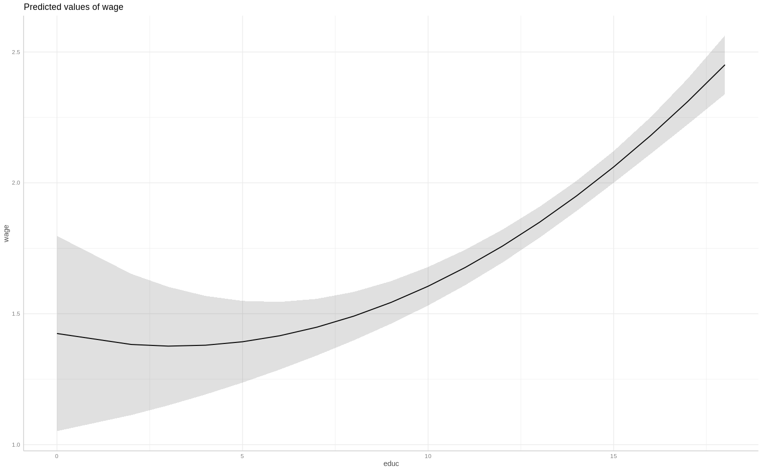

Code

ggpredict(fit_2, terms = "educ") %>% plot()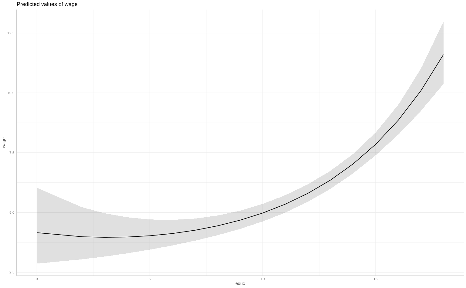

Code

ggpredict(fit_2, terms = c("educ", "sex")) %>% plot()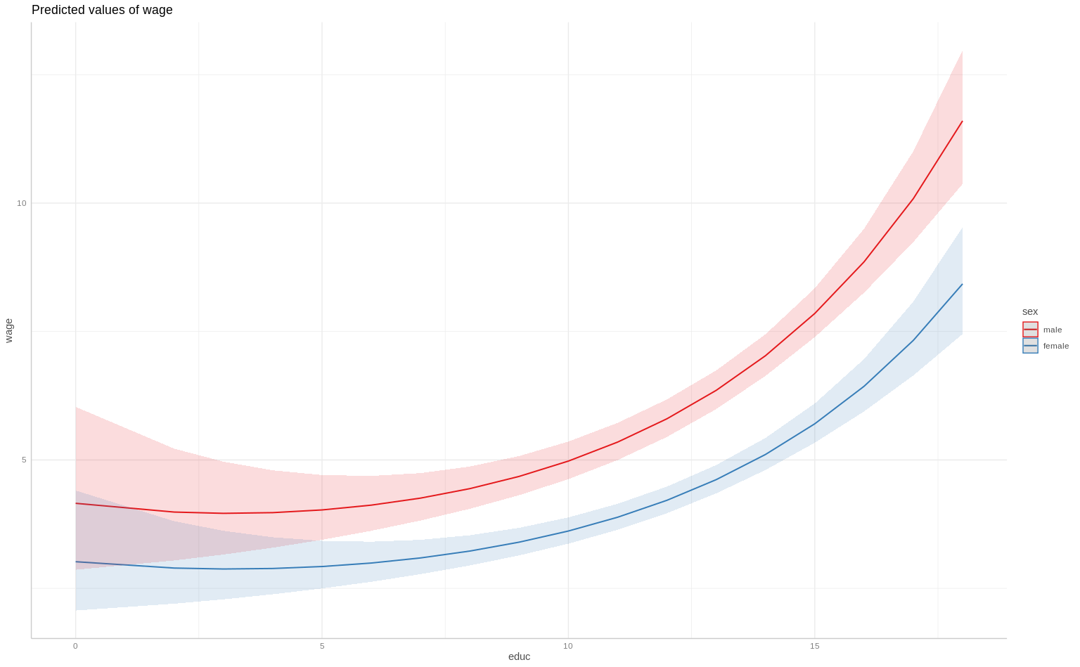

Code

# 1.8 Effect of a dummy variable
ggpredict(fit_2, terms = "sex") %>% plot()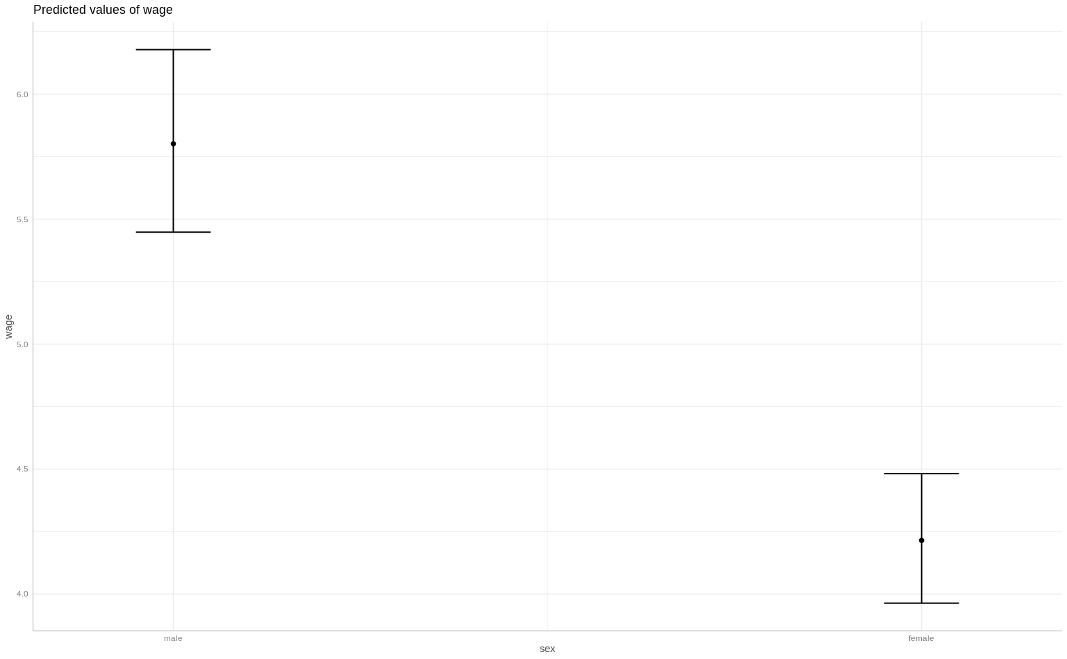

Code

ggpredict(fit_2, terms = "sex", back.transform = F)

# Predicted values of wage

sex    | Predicted |       95% CI
---------------------------------
male   |      1.76 | [1.70, 1.82]
female |      1.44 | [1.38, 1.50]

Adjusted for:
*  educ = 12.00
* exper = 13.50

Code

parameters(fit_2)

Parameter    | Coefficient |       SE |         95% CI | t(520) |      p
------------------------------------------------------------------------
(Intercept)  |        1.02 |     0.19 | [ 0.64,  1.39] |   5.32 | < .001
educ         |       -0.03 |     0.03 | [-0.09,  0.03] |  -1.00 | 0.316 
educ^2       |    4.87e-03 | 1.26e-03 | [ 0.00,  0.01] |   3.86 | < .001
exper        |        0.04 | 4.77e-03 | [ 0.03,  0.05] |   8.37 | < .001
exper^2      |   -7.19e-04 | 1.06e-04 | [ 0.00,  0.00] |  -6.76 | < .001
sex [female] |       -0.32 |     0.04 | [-0.39, -0.25] |  -8.84 | < .001

Code

# Exercise 2. Interaction term
## 2.1 Adding an interaction term between sex and education
fit_3 <- lm(log(wage) ~ 
              educ + I(educ ^ 2) + exper + I(exper ^ 2) + sex + 
              educ:sex, 
            data = dta)
parameters(fit_3)

Parameter           | Coefficient |       SE |         95% CI | t(519) |      p
-------------------------------------------------------------------------------
(Intercept)         |        1.06 |     0.21 | [ 0.65,  1.48] |   5.02 | < .001
educ                |       -0.04 |     0.03 | [-0.10,  0.03] |  -1.11 | 0.267 
educ^2              |    4.97e-03 | 1.28e-03 | [ 0.00,  0.01] |   3.89 | < .001
exper               |        0.04 | 4.77e-03 | [ 0.03,  0.05] |   8.37 | < .001
exper^2             |   -7.22e-04 | 1.07e-04 | [ 0.00,  0.00] |  -6.78 | < .001
sex [female]        |       -0.41 |     0.17 | [-0.74, -0.07] |  -2.37 | 0.018 
educ * sex [female] |    6.90e-03 |     0.01 | [-0.02,  0.03] |   0.51 | 0.608 

Code

performance(fit_3)

# Indices of model performance

AIC      |      BIC |    R2 | R2 (adj.) |  RMSE | Sigma
-------------------------------------------------------
2267.084 | 4008.885 | 0.417 |     0.410 | 0.406 | 0.408

Code

check_model(fit_3, check = c("linearity", "homogeneity"))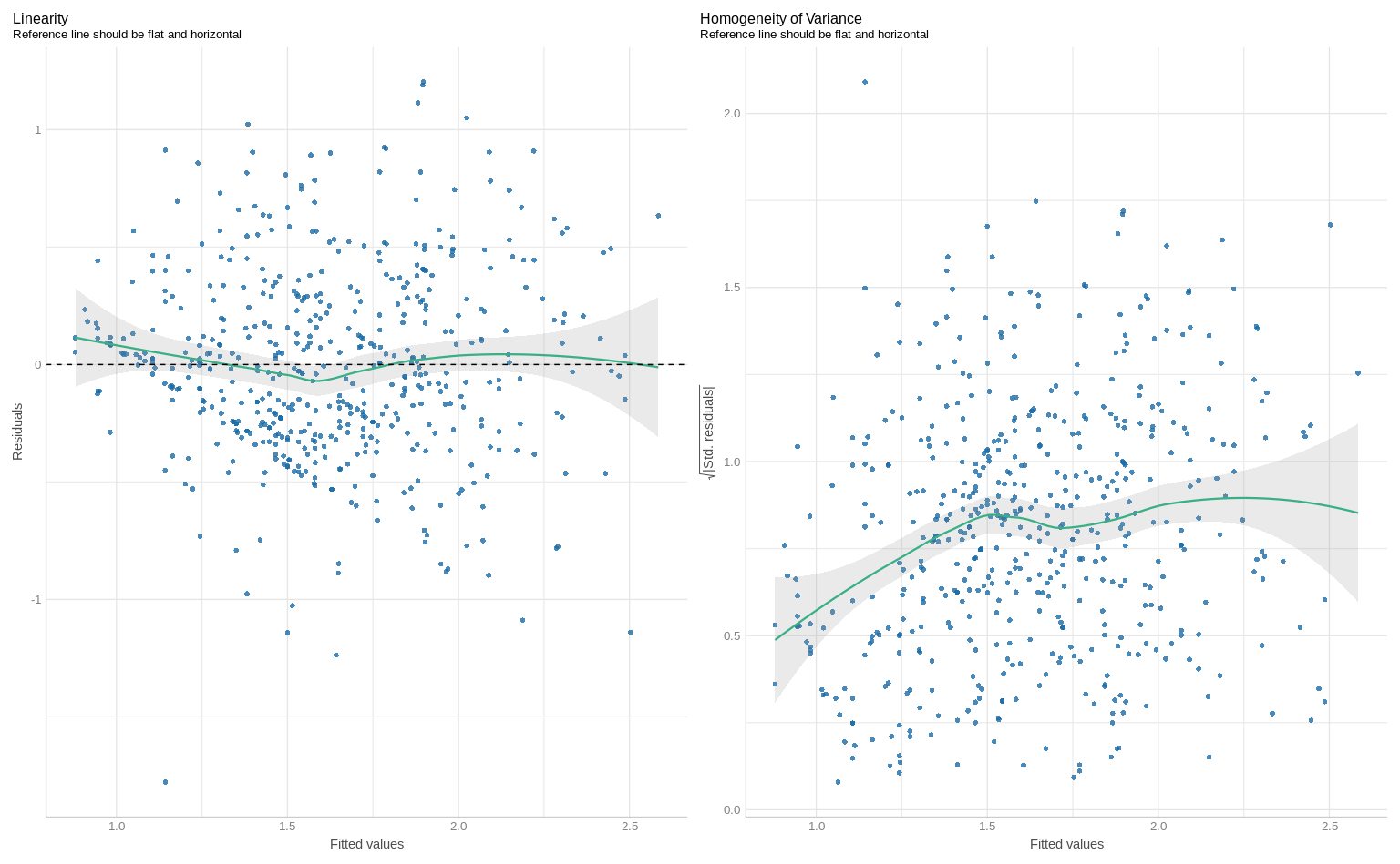

Code

## 2.2 Interpreting the interaction term
estimate_slopes(fit_3, trend = "educ", at = "educ") %>% plot()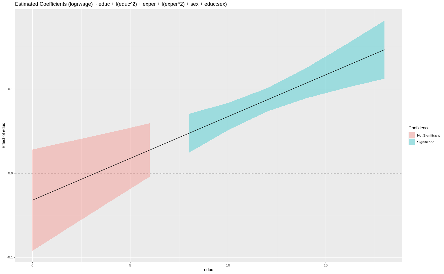

Code

estimate_slopes(fit_3, trend = "educ", at = c("sex", "educ")) %>% plot()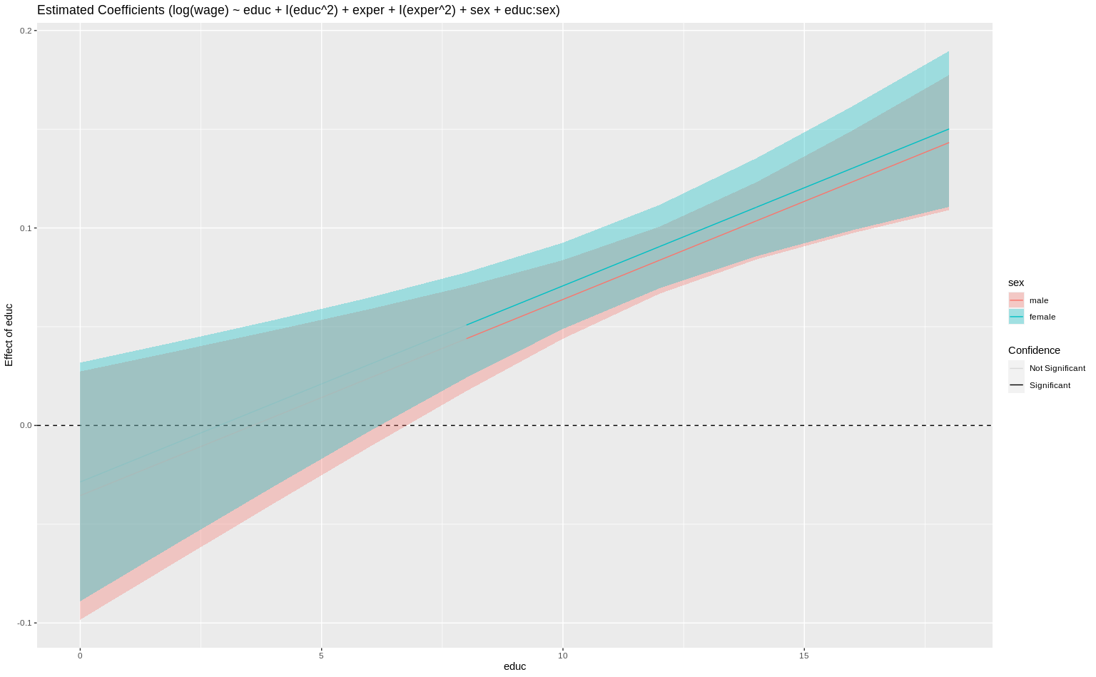

Code

estimate_slopes(fit_3, trend = "educ", at = c("sex")) %>% plot()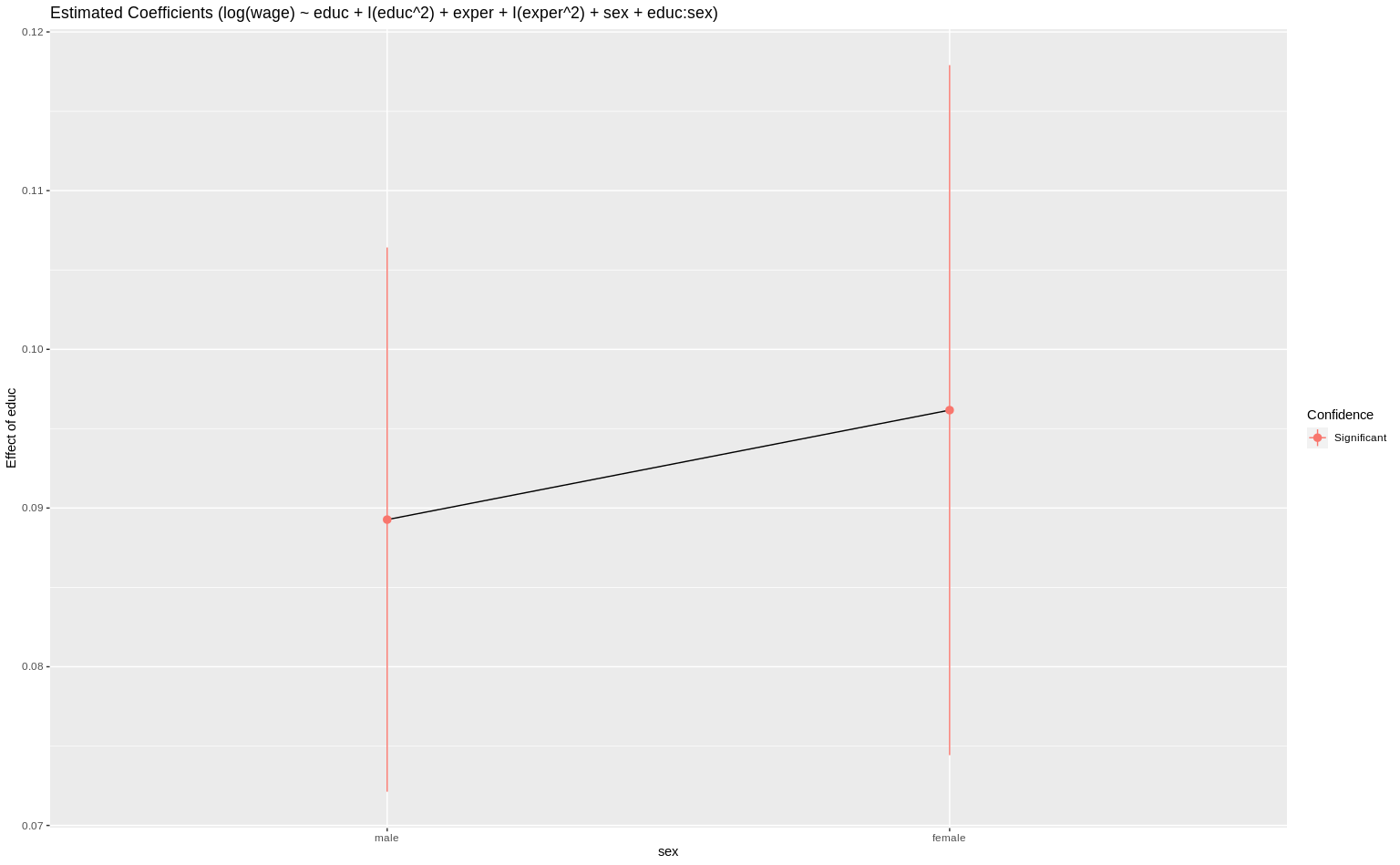

Code

ggpredict(fit_3, terms = "educ") %>% plot()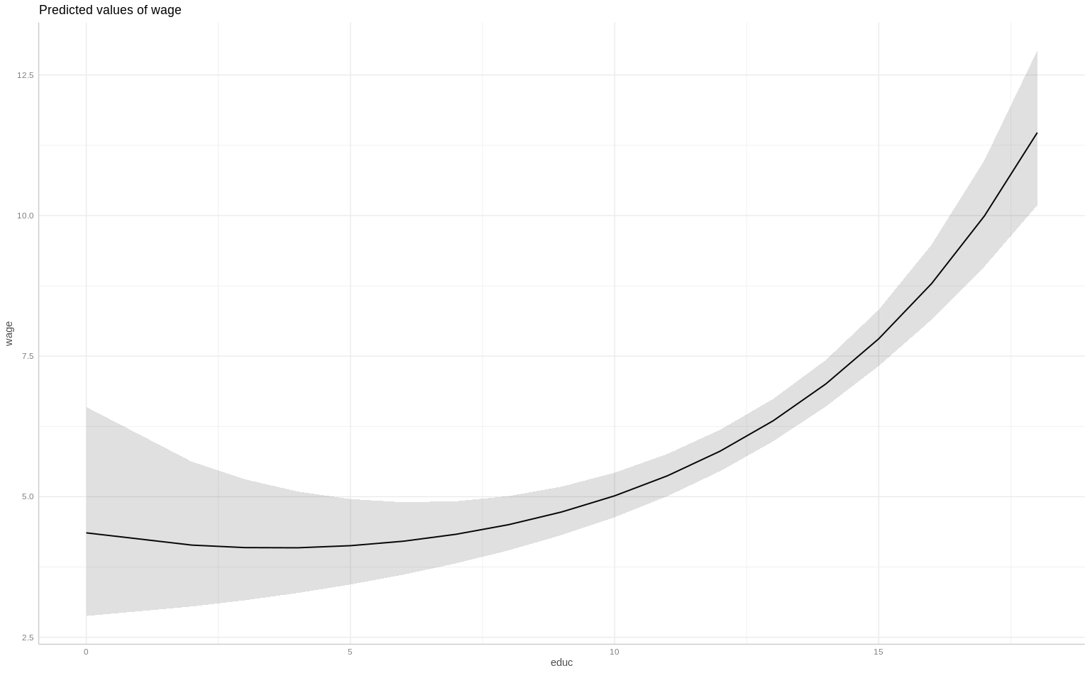

Code

ggpredict(fit_3, terms = c("sex", "educ")) %>% plot()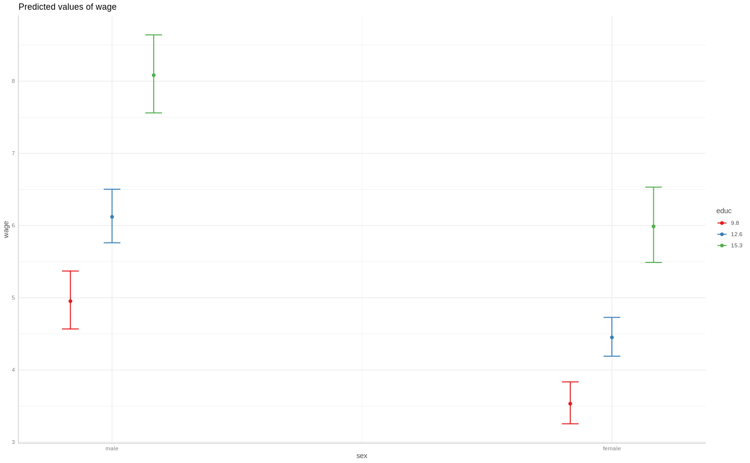

Code

ggpredict(fit_3, terms = c("educ", "sex")) %>% plot()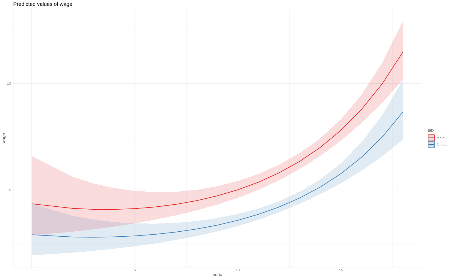

Code

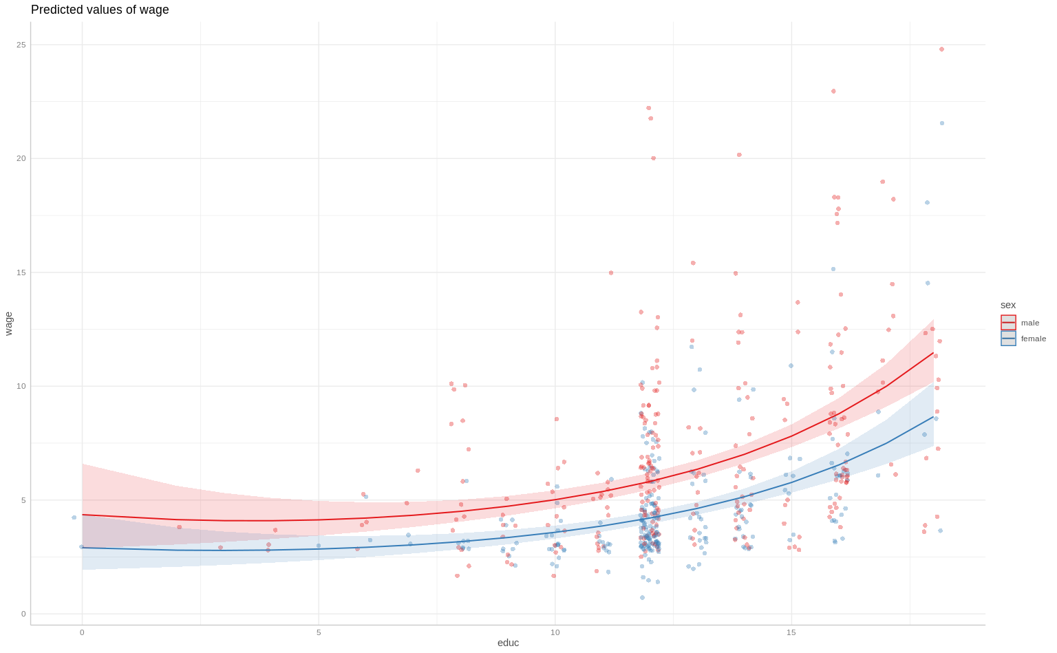
ggpredict(fit_3, terms = c("educ", "sex")) %>% plot(add.data = TRUE)