Regression Discontinuity Design

Eduard Bukin

Regression Discontinuity (Design)

  • Exploit natural experiments that constrain the role of chance in human affairs by arbitrary decision-making in policy that divide groups.

  • Rigid rules that aim to eliminate randomness create a natural experiment with the random components.

  • There area: Sharp and Fuzzy RDD

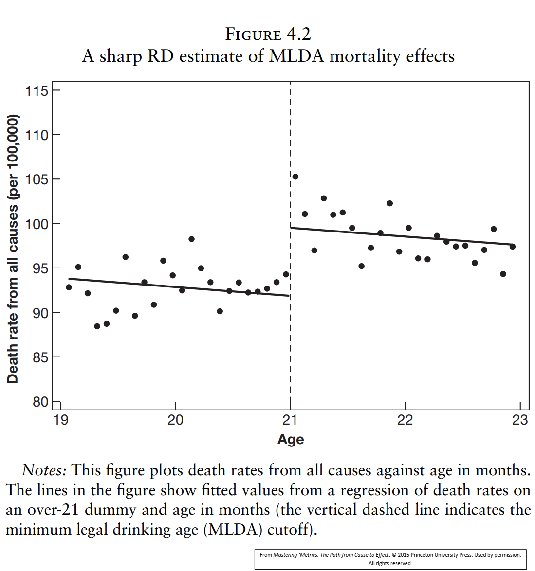
Example 1. Birthdays and funerals (Angrist & Pischke, 2014)
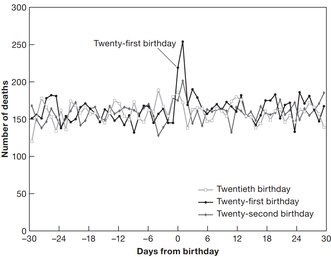
  • After the 21st birthday, the number of death spikes in the USA.

  • Why?

  • In the number of death over age, there is some kind of discontinuity.

Theoretical basis

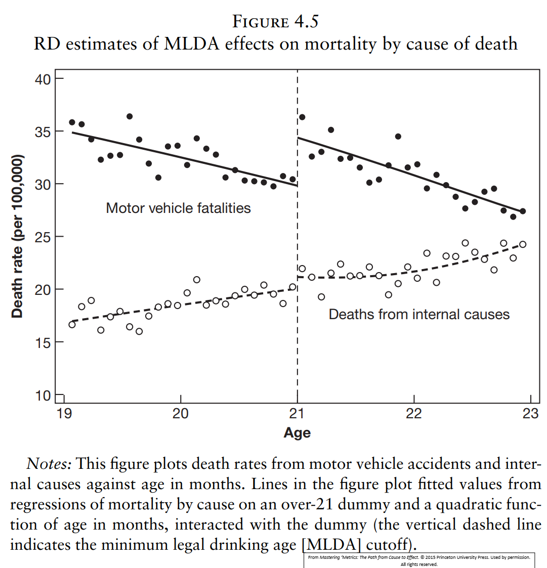
  • Yong people are more likely to die from external causes such as car accidents or suicides.

  • Older people are more likely to die from internal causes (cancer).

Discontinuity in the death rate over age must be caused by some external factors.

  • Policy.

Regression Discontinuity (Design) RDD is called like that because it uses regression to determine the discontinuity.

RDD: basics

  • \(a\) age of the cohort of people;
  • \(\bar M_a\) as the monthly average death rate for the cohort;
  • \(D_a\) dummy variable that indicates if the cohort \(a\) has right to drink alcohol.

\[ D_{a}= \begin{cases} 1, & \text{if}\ a \ge 21 \\ 0, & \text{if}\ a < 21. \end{cases} \]

Treatment status \(D_a\) is discontinuous of the running variable \(a\) at the cut-off threshold \(21\).

Using regression we can estimate the effect of the discontinuity \(\rho\):

\[ \bar M_{a} = \alpha + \rho D_a + \gamma a + e_a, \]

where

  • \(\rho\) captures the jump in death due to the policy change,

  • \(\gamma\) reflects internals/external causes substitution.

RDD: anatomy

\[ \bar M_{a} = \alpha + \rho D_a + \gamma a + e_a, \]

  • This is a short model.

    • Does it suffer from the OVB?
  • No, because:

    • treatment \(D_a\) depends only on \(a\), and

    • there is no difference between 20 and 21 yo

    • there is no difference between 20 years and 11 m.o. and 21y. and 1 m.o.

    • we have “insiders” information about the similarity of the observations on two sides of the treatment/threshold.

Sharp vs Fuzzy RDD

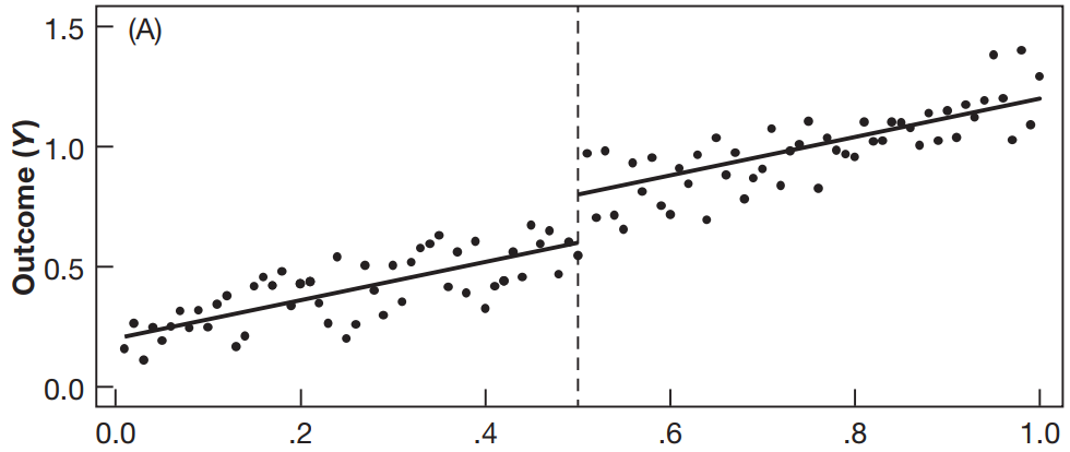
Sharp: the threshold is sharp and changes status from one to another immediately.

  • \(a\) is age and age limit is a threshold that

  • probability of treatment changes from 0 to 1 at the threshold.

Fuzzy RDD:

  • Probability of intensity of treatment usually persists all along the running variables,

  • but at the cut-off probability of treatment intensity jumps.

RDD: visual transparency

RDD: robustness
RDD: limitations

  • External validity:

  • Non-linear relationship between running variable and discontinuity:

  • Discontinuity must be sharp but it may not be observed in the data.

RDD: bandwidth

Window around the threshold that we use to estimate the effect of the cut-off.

  • bandwidth is the trade-off between Bias and Variance.

  • Selecting bandwidth

    • bandwidth should vary as a function of the sample size: more information, narrower the bandwidth.

    • Point of the judgment call, but results should be robust given the bandwidth variation.

See Imbens & Kalyanaraman (2011)

Non linearity and discontinuity (1)

Non linearity and discontinuity (2)
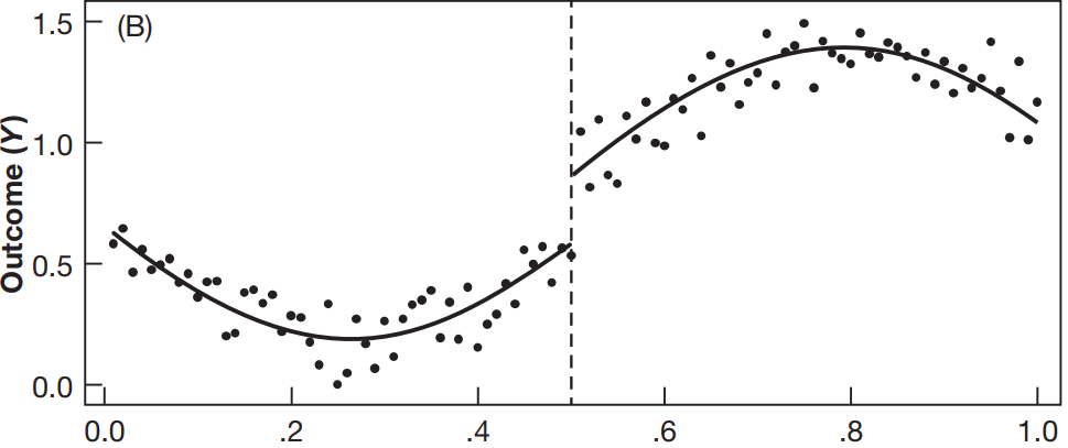
Non linearity and discontinuity (3)
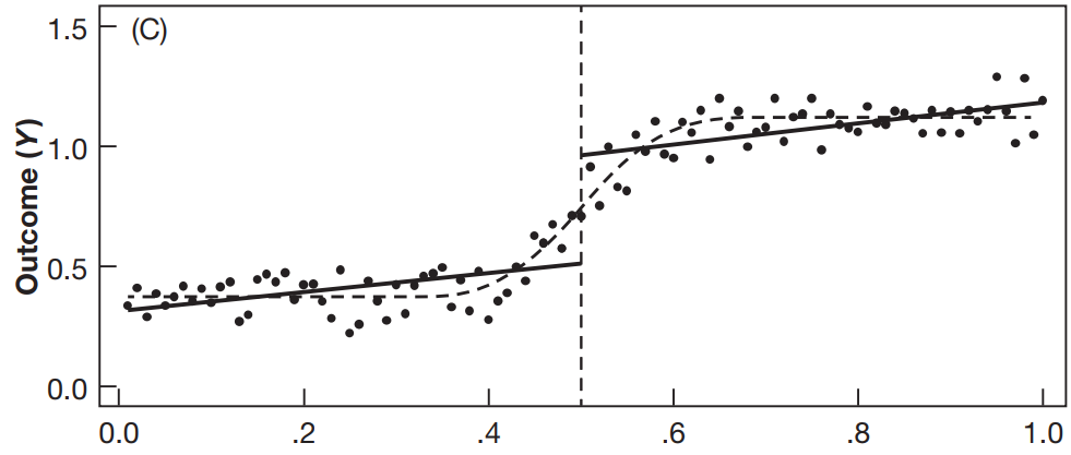
Non linearity solutions

  1. Polynomial:
  • \(\bar M_{a} = \alpha + \rho D_a + \gamma_1 a + \gamma_2 a^2 + e_a\)
  • could be too good and confirm prejudices;
  • we need to make a judgment call in a publication and check alternatives with robustness checks.
  1. Centering the running variable at the cut-off \(a_0\) and adding the interaction term with \(D_a\).
  • \(\bar M_{a} = \alpha + \rho D_a + \gamma (a - a_0) + \delta [(a-a_0)D_a] + e_a\)
  • When centered, \(\rho\) is the the jump parameter.
  • change in the slope of \(\rho\) before and after the threshold with: \(\rho + \delta (a - a_0)\).
  1. Non linearity and the cut-off slope change could be combined:
  • \(\bar M_{a} = \alpha + \rho D_a + \gamma_1 (a - a_0) + \gamma_2 (a - a_0) ^ 2 + \delta_1 [(a-a_0)D_a] + \delta_2 [(a-a_0) ^ 2 D_a] + e_a\)

Complexity vs simplicity

  • No general rule on choosing one or another model (simple vs complex);

  • Better to have robust not-sensitive results.

  • Visual inspection is a key.

  • Checks and balances are important. Check for the composites of the death for example.

  • There are also non-parametric approaches.

Difference of the RD from the regression

  • In the regression we control for other factors

    • hoping that this will match counterfactual for our factual and ensure the ceteris paribus.
  • In the RDD running variable \(a\) is the one that ensures that:

    • once we can observe the treatment we cannot observe the counterfactual.
  • It works at least for the observations that are neighboring on the running variable.

RDD in agricultural and environmental economics

See: (Wuepper & Finger, 2022)

Specific considerations:

  1. Ag economics may rely on remote sensing and GIS data more.

  2. Distances from physical borders or longitude and latitude coordinates are the running variables

East or West Germany, farm size and biodiversity (Noack, Larsen, Kamp, & Levers, 2021)
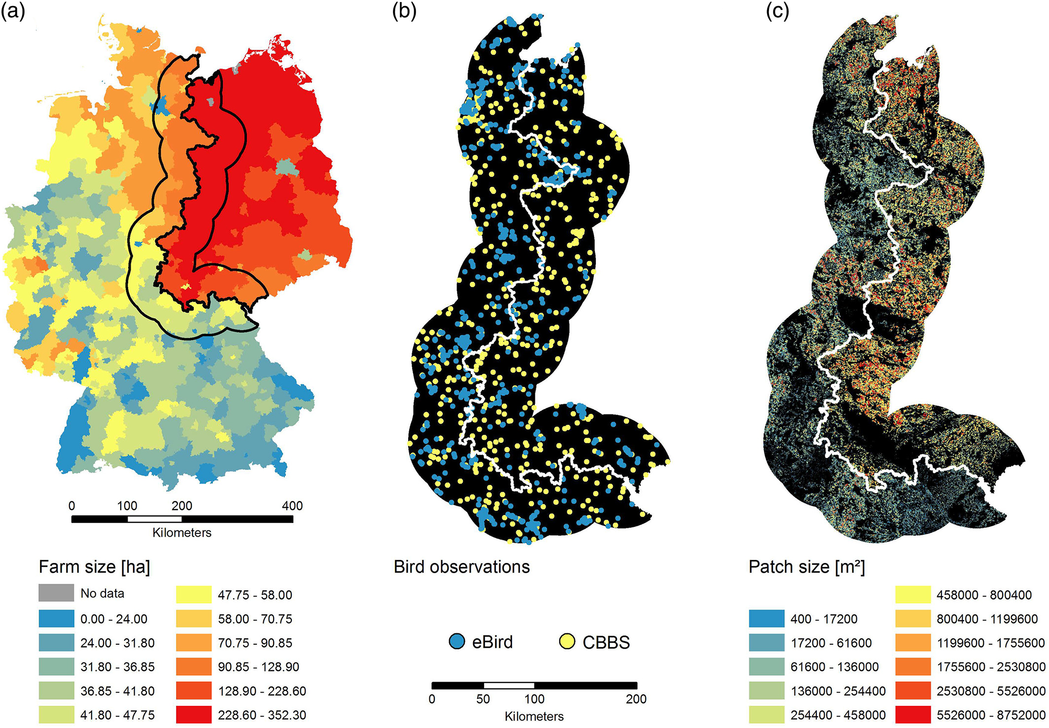
East or West Germany: farm size (Noack et al., 2021)
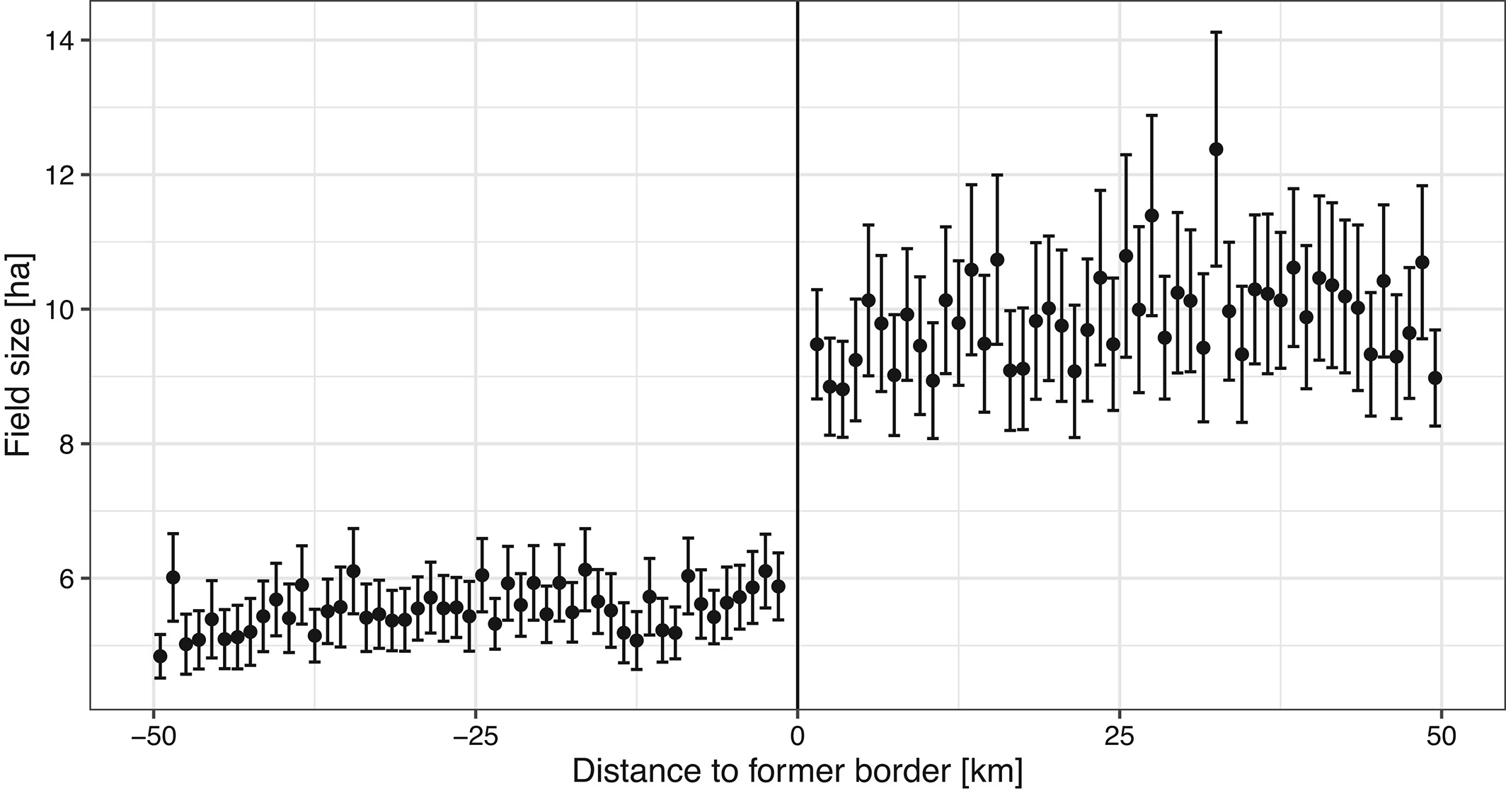
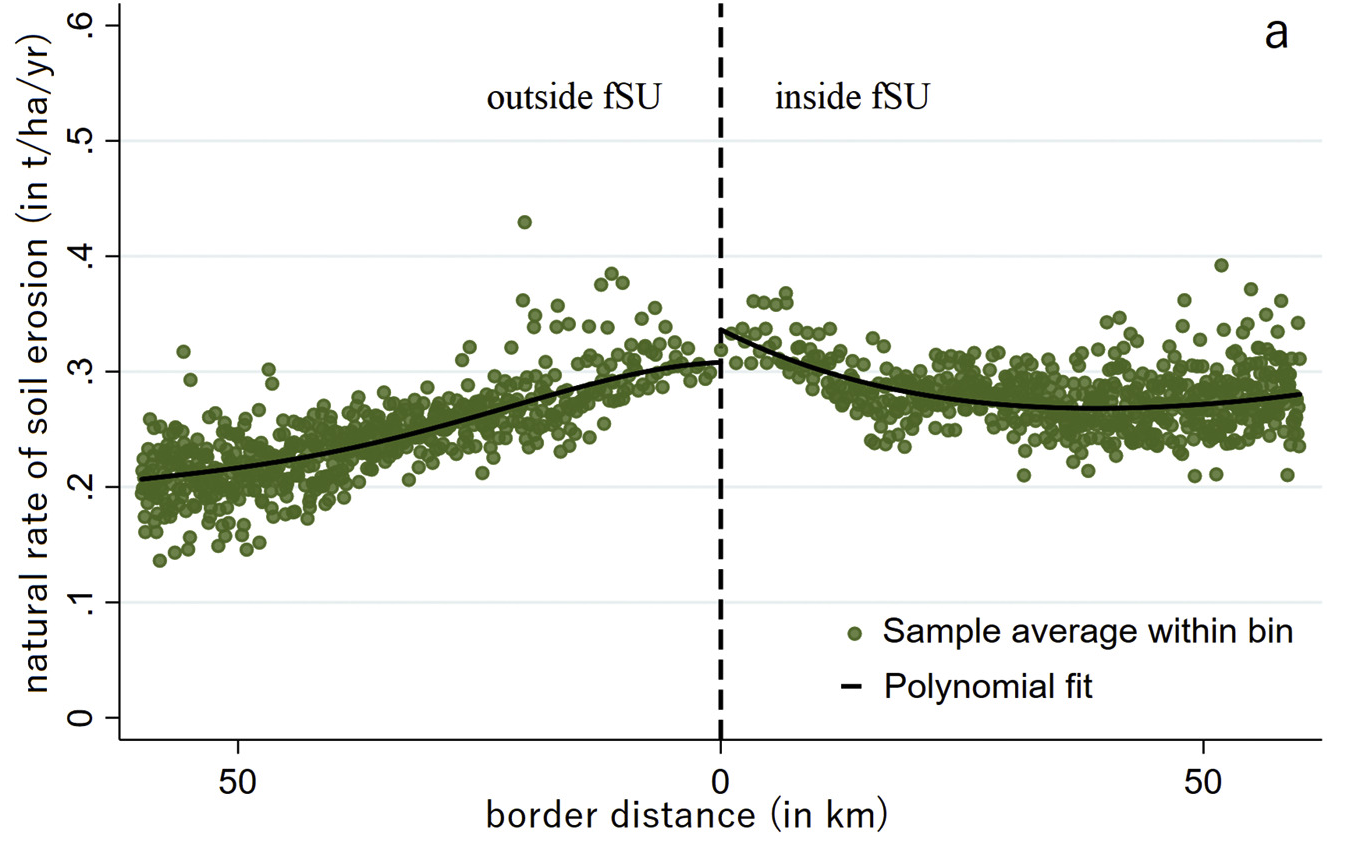
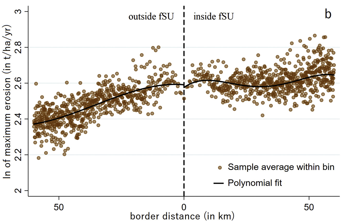
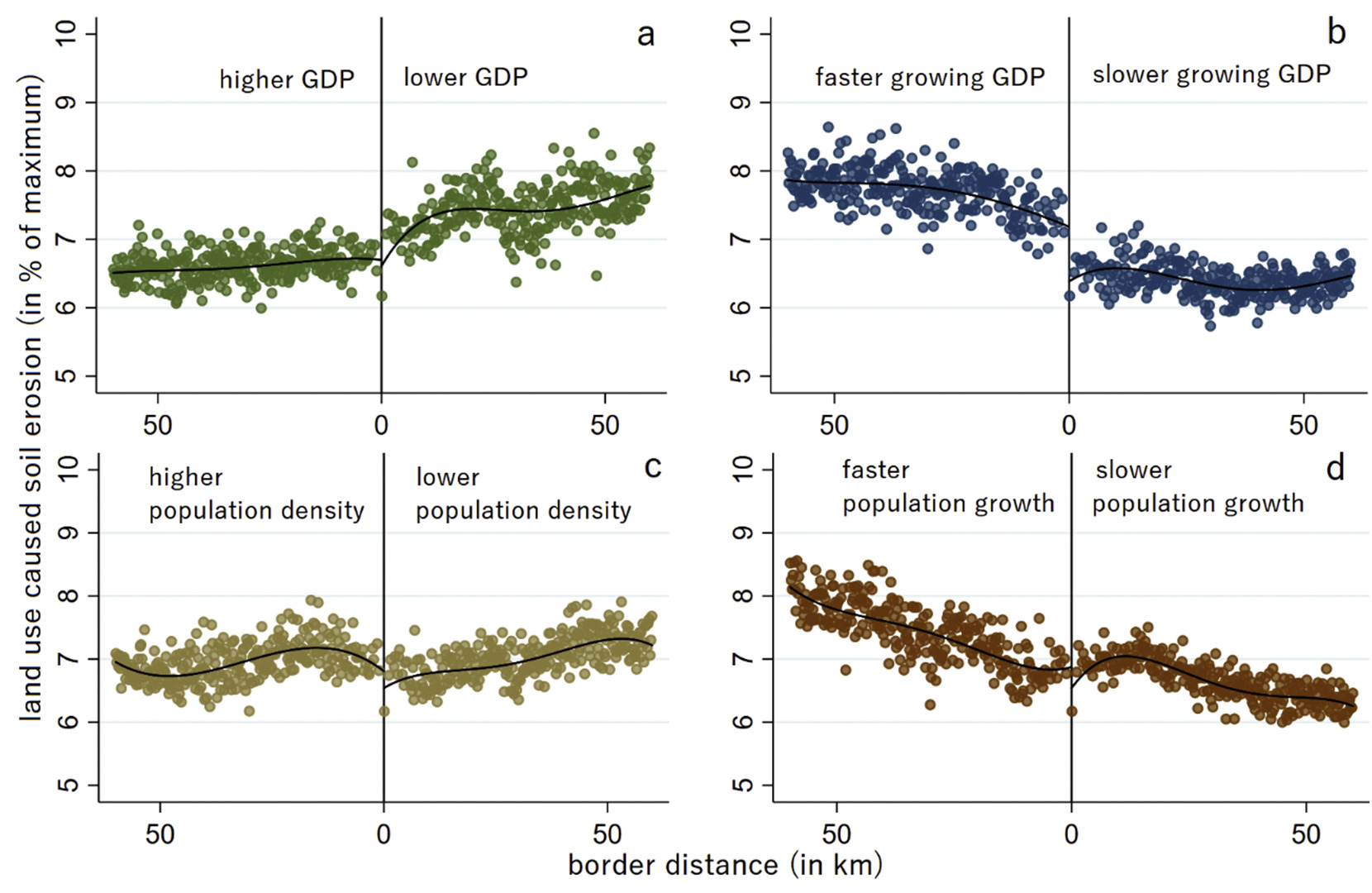
Soil erosion and the Soviet legacy (Wuepper, Borrelli, Mueller, & Finger, 2020)
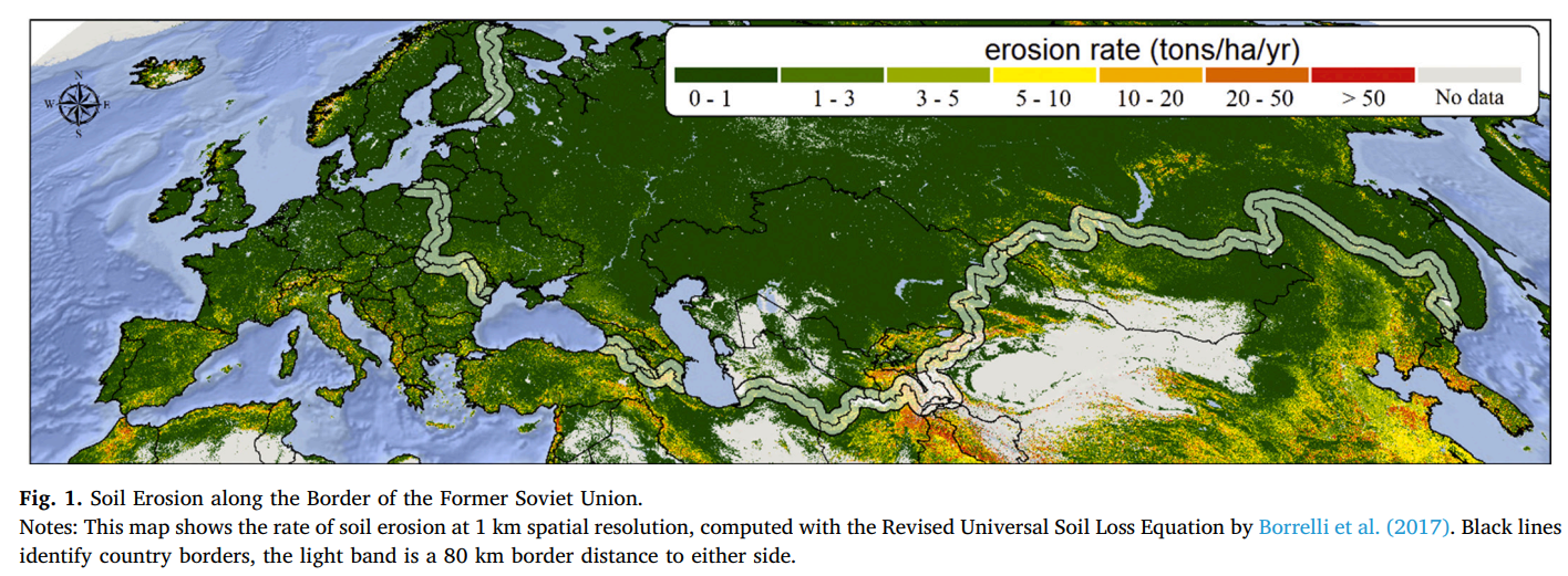
Wuepper et al. (2020): Natural soil erosion
Wuepper et al. (2020): Maximum soil erosion
Wuepper et al. (2020): Soil erosion due to land use

Wuepper et al. (2020): Robustness checks
Wuepper et al. (2020): Forest cover
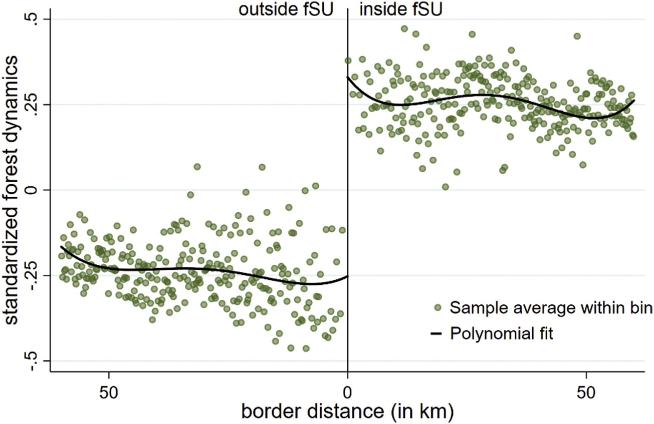
Wuepper et al. (2020)

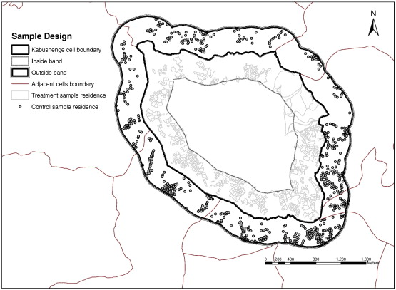
Sampling strategy in (Ali, Deininger, & Goldstein, 2014)
More examples and practice

< https://rdpackages.github.io >

References

Ali, D. A., Deininger, K., & Goldstein, M. (2014). Environmental and gender impacts of land tenure regularization in africa: Pilot evidence from rwanda. Journal of Development Economics, 110, 262–275. http://doi.org/10.1016/j.jdeveco.2013.12.009
Angrist, J. D., & Pischke, J.-S. (2014). Mastering’metrics: The path from cause to effect. Princeton University Press.
Imbens, G., & Kalyanaraman, K. (2011). Optimal bandwidth choice for the regression discontinuity estimator. The Review of Economic Studies, 79(3), 933–959. http://doi.org/10.1093/restud/rdr043
Noack, F., Larsen, A., Kamp, J., & Levers, C. (2021). A birds eye view of farm size and biodiversity: The ecological legacy of the iron curtain. American Journal of Agricultural Economics, 104(4), 1460–1484. http://doi.org/10.1111/ajae.12274
Wuepper, D., Borrelli, P., Mueller, D., & Finger, R. (2020). Quantifying the soil erosion legacy of the soviet union. Agricultural Systems, 185, 102940. http://doi.org/10.1016/j.agsy.2020.102940
Wuepper, D., & Finger, R. (2022). Regression discontinuity designs in agricultural and environmental economics. European Review of Agricultural Economics, 50(1), 1–28. http://doi.org/10.1093/erae/jbac023