Panel Regression Analysis: Micro application to production function

Eduard Bukin

Example 2. Micro-level application of panel regression analysis `RiceFarms`

Are larger farms more productive if compared to the smaller once?
This example:
- explores relationship between farm size and productivity.
- guides through the process of panel regression analysis.

Part 1. Theoretical basis

We employ the Cobb-Douglas Production function:

\[ \ln y = \ln \beta_0 + \sum_{n = 1}^{N} \beta_n \ln x_n + \sum_{k = 1}^{K} \gamma_k \delta_k + \epsilon \]

where,

\(y\) is the output and \(x_n\) are the inputs all in physical mass (or monetary value);
\(N\) is the number of independent variables;
\(\delta_k\) are the shift parameters of additional dummy variables;
\(\beta_0\) , \(\beta_n\) , \(\gamma_n\) are the estimated coefficients;

Estimation strategy. Part 1.

Pooled OLS production function:

\[ \begin{aligned} \ln \text{output}_{it} & = A_0 + \beta_1 \cdot \ln \text{land}_{it} + \beta_2 \cdot \ln \text{labor}_{it} \\ & + \beta_3 \cdot \ln \text{seed}_{it} + \beta_4 \cdot \ln \text{urea}_{it} \\ & + \beta_5 \cdot \ln \text{pesticide}_{it} + e_{it} \end{aligned} \]

What are the ex-ante expectations about the regression coefficients?
- Ideas? …
- Probably all \(\beta\) should be positive.

What about OVB?

What omitted variables could cause bias of our estimates?

Any!? …
Any!? …
Any OVB!? …
Capital, Ability, Climate, Geography…

Using the OVB formula

Let us make an educated guess about the effect of OVB on the estimates of land-related coefficient \(\beta_1\)?

Short:
Long:
Aux.
OVB:

\(\text{output}_{it} = A_0^s + \beta_1^s \cdot \text{land}_{it} + \beta_2^s \cdot \text{labor}_{it} + \beta_3^s \cdot \text{seed}_{it} + \beta_4^s \cdot \text{urea}_{it} + \beta_5^s \cdot \text{pesticide}_{it} + e_{it}\)
\(\text{output}_{it} = A_0 + \beta_1 \cdot \text{land}_{it} + \beta_2 \cdot \text{labor}_{it} + \beta_3 \cdot \text{seed}_{it} + \beta_4 \cdot \text{urea}_{it} + \beta_5 \cdot \text{pesticide}_{it} + \color{Red}{\gamma \text{Ability}_i} + e_{it}\)
\(\text{Ability}_i = \pi_0 + \color{Blue}{\pi_1 \cdot \text{land}_{it}} + \pi_2 \cdot \text{labor}_{it} + \pi_3 \cdot \text{seed}_{it} + \pi_4 \cdot \text{urea}_{it} + \pi_5 \cdot \text{pesticide}_{it} + e_{it}\)
\(\text{OVB}_{\text{land}} = \beta_1^s - \beta_1 = \color{Red}{\pi_1} * \color{Blue}{\gamma}\)

Educated guess about the bias of the estimates.
What are the signs of \(\pi_1\) and \(\gamma\)?
- \(\pi_1 > 0\)
- \(\gamma > 0\)
- \(\text{OVB} = (+) \times (+) > 0\)
Not controlling for the OV \(\text{ability}_i\) may cause overestimation of the effect of the farm size \(\beta_1\).
\(\text{ability}_i\) does not vary over time for each farm!

How to resolve such OVB?

Introduce a proxy variable for ability?
- No such data.
Rely on the panel structure of the data.
- Use the individual fixed effect model, for example.

Estimation strategy. Part 2.

Individual fixed effect panel regression production function.

What are the ex-ante expectations about the regression coefficients?
- Ideas? …
- Probably the same as before: all \(\beta\) should be positive.

Estimation strategy. Part 3. Return to scale (1)

Are larger farms more productive?

To understand this, we need to calculate how joint increase of all inputs change the output.

If increase of all inputs by 1% increases output also by the same 1%, we have a constant return to scale.
If increase of all inputs by 1% increases output also by more than 1%, we have an increasing return to scale.
If increase of all inputs by 1% increases output also by less than 1%, we have an decreasing return to scale.

Estimation strategy. Part 3. Return to scale (2)

From the main equation,

return to scale can be estimated as a sum of all coefficients:

\[ \text{Rreturn to scale} = \beta_1 + \beta_2 + \beta_3 + \beta_4 + \beta_5 \]

To perform a hypothesis testing about the return to scale, we need to employ:
- HT about a linear combination of parameters, and
- delta method for estimating standard errors.

Estimation strategy. Part 3. Return to scale (3)

HT about a linear combination of parameters:

H0 - \(\beta_1 + \beta_2 + \beta_3 + \beta_4 + \beta_5 = 1\) (also can be \(=0\) or any number)
H1 - \(\beta_1 + \beta_2 + \beta_3 + \beta_4 + \beta_5 \ne 1\) (also can be \(\ne0\) or any number)

We compute standard errors using delta method (car::deltaMethod()).

And perform HT using F statistics.

Part 2. Exploratory data analysis and data description

We operate a farm-level data with following variables:

output - gross output of rice in kg
land - the total area cultivated with rice, measured in hectares
seed - seed in kilogram
urea - urea in kilogram
pesticide - urea in kilogram
labor - total labor in hours (excluding harvest labor)

Data preparation

Load data and calculate rice yields and logs of all variables.

library(tidyverse)
library(plm)
library(modelsummary)
library(performance)
library(lmtest)

farm_dta <- read_csv("farm_panel.csv")

glimpse(farm_dta)

Rows: 1,026
Columns: 15
$ id         <dbl> 101001, 101001, 101001, 101001, 101001, 101001, 101017, 101…
$ time       <dbl> 1999, 2000, 2001, 2002, 2003, 2004, 1999, 2000, 2001, 2002,…
$ output     <dbl> 7980, 4083, 2650, 4500, 16300, 17424, 3840, 2800, 950, 240,…
$ land       <dbl> 3.000, 2.000, 1.000, 2.000, 3.572, 3.572, 1.420, 1.420, 0.4…
$ labor      <dbl> 2915, 2155, 1075, 2091, 3889, 3519, 810, 855, 460, 109, 230…
$ hiredlabor <dbl> 2875, 2110, 980, 2081, 3889, 3519, 670, 805, 380, 40, 210, …
$ famlabor   <dbl> 40, 45, 95, 10, 1, 1, 140, 50, 80, 69, 20, 1, 108, 63, 57, …
$ seed       <dbl> 90, 40, 100, 60, 105, 105, 50, 20, 15, 7, 15, 15, 5, 10, 10…
$ urea       <dbl> 900, 600, 700, 600, 400, 400, 120, 100, 150, 50, 100, 100, …
$ pest       <dbl> 6000, 3000, 5000, 5000, 10200, 10200, 0, 0, 900, 0, 2000, 2…
$ varieties  <chr> "mixed", "trad", "high", "high", "high", "high", "trad", "h…
$ status     <chr> "owner", "owner", "owner", "owner", "share", "share", "mixe…
$ bimas      <chr> "mixed", "mixed", "mixed", "mixed", "no", "no", "mixed", "m…
$ region     <chr> "wargabinangun", "wargabinangun", "wargabinangun", "wargabi…
$ price      <dbl> 60, 60, 65, 70, 120, 140, 60, 50, 62, 60, 110, 130, 65, 50,…

Computing yields and logs

farm_dta_log <- farm_dta %>%
  mutate(
    l_output = log(output),
    l_land = log(land),
    l_seed = log(seed),
    l_urea = log(urea),
    l_pest = log(pest),
    l_labor = log(labor),
    yields_mt_ha = output / land / 1000
  )

Summary statistics

n_inf <- function(x) sum(is.infinite(x))
n_missing <- function(x) sum(is.na(x)|is.nan(x))
datasummary(
  l_output + l_land + l_seed + l_urea + l_pest + l_labor + yields_mt_ha ~ 
    N + n_missing + n_inf + Mean + SD + Median + Min + Max,
  data = farm_dta_log)

	N	n_inf	Mean	SD	Median	Min	Max
l_output	1026	0.00	6.73	0.99	6.79	3.74	9.95
l_land	1026	0.00	−1.30	0.95	−1.25	−4.61	1.67
l_seed	1026	0.00	2.37	0.94	2.30	0.00	7.13
l_urea	1026	0.00	3.98	1.16	4.09	0.00	7.13
l_pest	1026	713.00					11.04
l_labor	1026	0.00	5.56	0.85	5.53	2.83	8.47
yields_mt_ha	1026	0.00	3.38	1.68	3.16	0.40	27.50

Any problems with data?

Any problems with data?

Any? …
pest, when transformed with logs, produces -Inf values.
- Why is that so?
- Any? …
- Because there are zero values of pesticides application \(\ln 0 = - \infty\).
How to resolve the \(\ln 0\) problem?

`-Infinity` in logs: lazy solution

Before log transformation, substitute any zero with a small value, for example 0.0001;

farm_dta_log <- farm_dta_log %>%
  mutate(l_pest_lazy = ifelse(is.infinite(l_pest), log(0.0001), l_pest))

`-Infinity` in logs: smart solution

Introduce reverse dummy variables for each variable with log of zero, see: Battese (1997);
Substitute negative infinity with zero. . . .

farm_dta_log <- farm_dta_log %>%
  mutate(pest_revdum = ifelse(is.infinite(l_pest), 1, 0),
         l_pest_smart = ifelse(is.infinite(l_pest), 0, l_pest))

Summary statistics after data cleaning

datasummary(l_pest + l_pest_lazy + l_pest_smart +  pest_revdum ~ 
    N + n_missing + n_inf + Mean + SD + Median + Min + Max, 
    data = farm_dta_log)

	N	n_inf	Mean	SD	Median	Min	Max
l_pest	1026	713.00					11.04
l_pest_lazy	1026	0.00	−4.37	7.35	−9.21	−9.21	11.04
l_pest_smart	1026	0.00	2.04	3.15	0.00	0.00	11.04
pest_revdum	1026	0.00	0.69	0.46	1.00	0.00	1.00

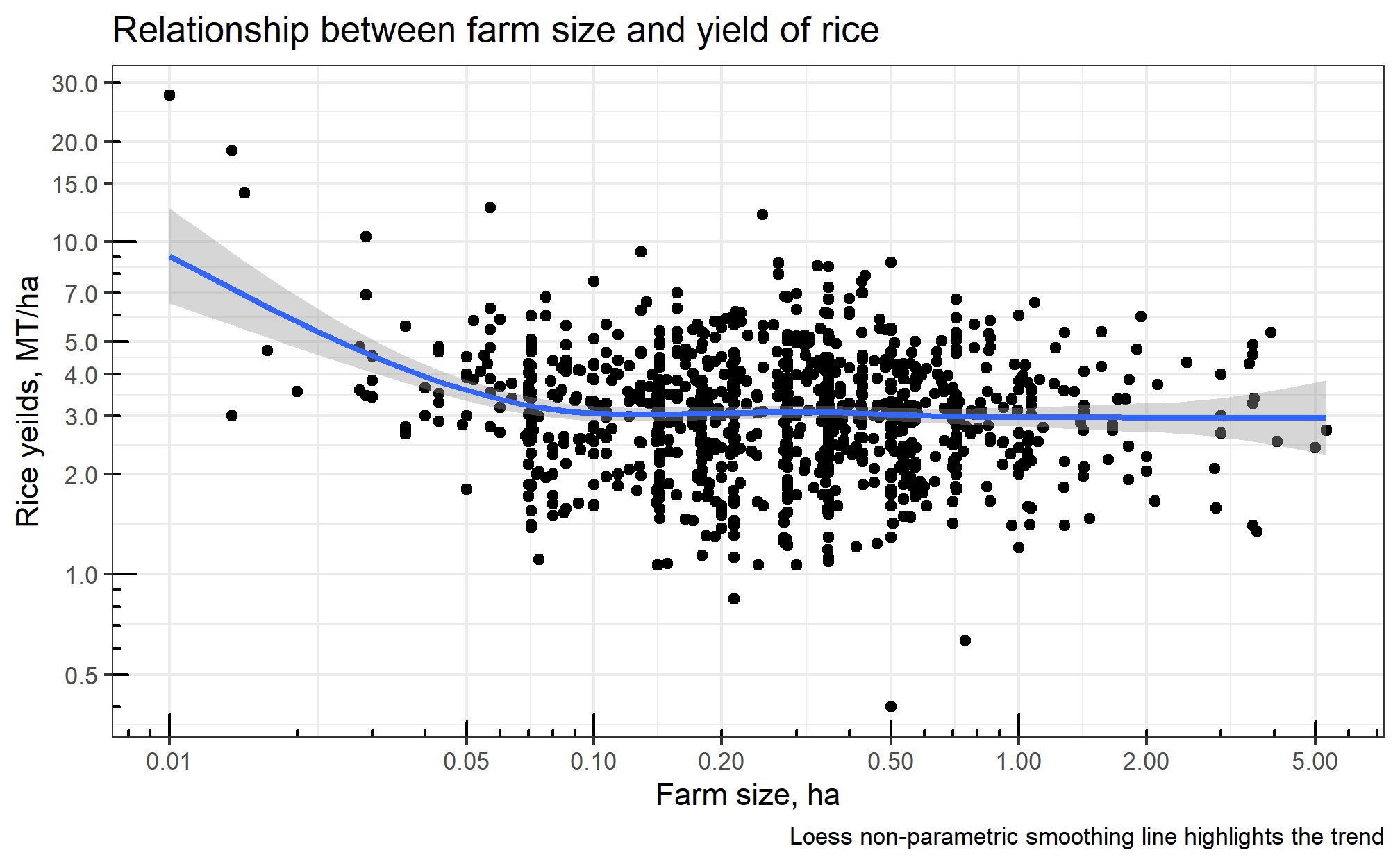
Farm size vs rice yields

yield_size <- 
  farm_dta_log %>% 
  ggplot() + 
  aes(x = land, y = yields_mt_ha) + 
  geom_point() + 
  geom_smooth() + 
  scale_x_log10("Farm size, ha", 
                breaks = c(0.01, 0.05, 0.1, 0.2, 0.5, 1, 2, 5, 10)) + 
  scale_y_log10("Rice yeilds, MT/ha", 
                breaks = c(0.2, 0.5, 1, 2, 3, 4, 5, 7, 10, 15, 20, 30)) + 
  annotation_logticks() + 
  labs(title = "Relationship between farm size and yield of rice",
       caption = "Loess non-parametric smoothing line highlights the trend")
yield_size

Farm size vs rice yields

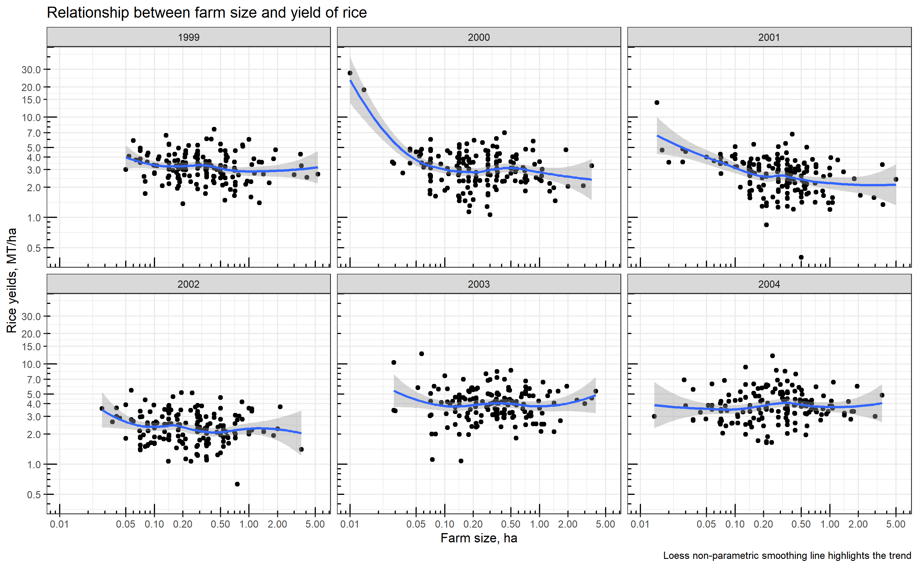
Farm size vs rice yields by year

yield_size + facet_wrap(. ~ time)

Part 3. Estimating the models

Step 1. Pooled OLS (with lm() and plm() functions);

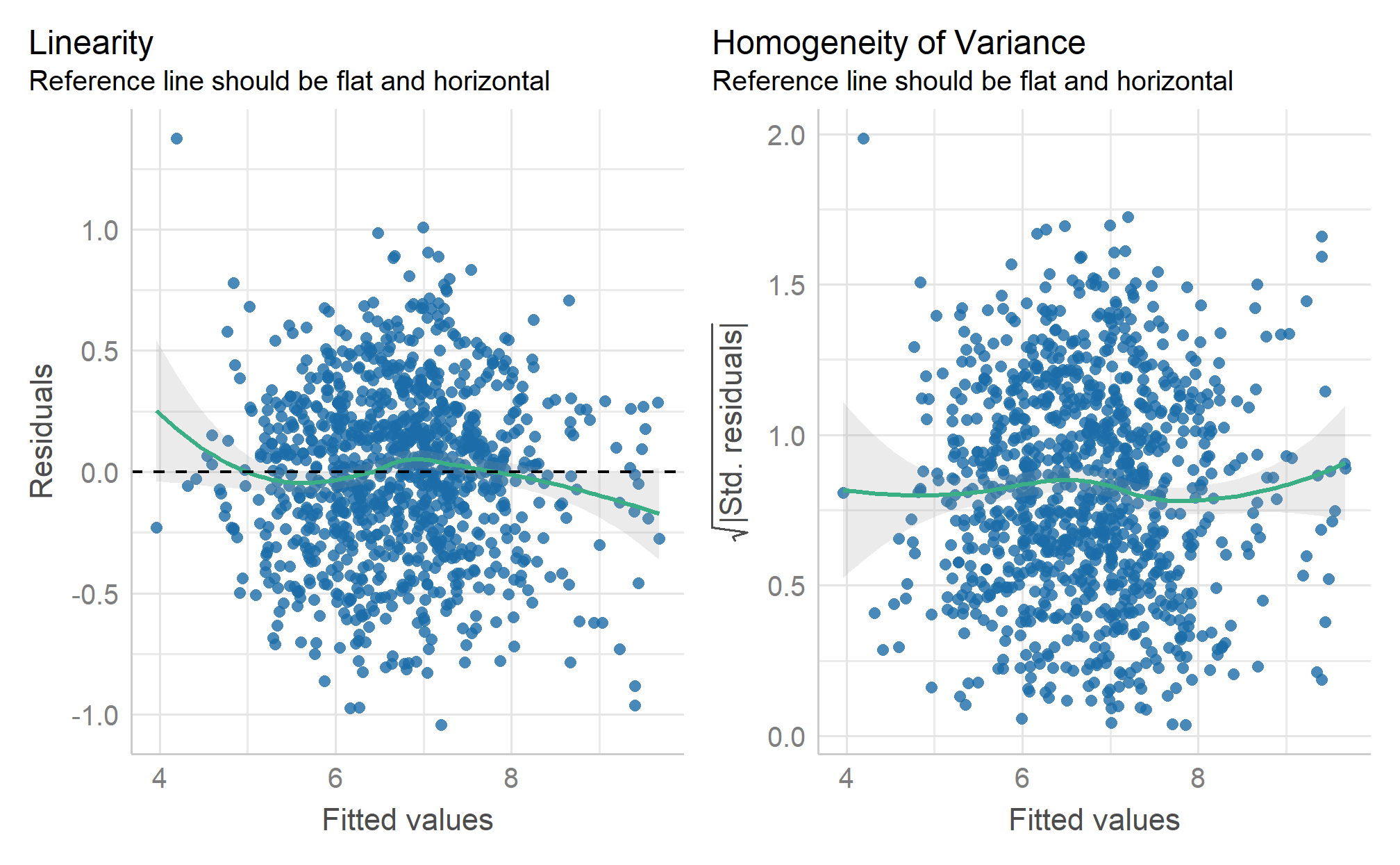
Validate all assumptions (linearity, collinearity, homogeneity)

Step 2. Fixed Effect and Random Effect models (with plm());

Choose a consistent model (models) relying on: F-test (pftest()), Lagrange multiplier test (plmtest()), Hausman test (phtest());

Step 3. Validate homogeneity assumption (cross-sectional dependency and autocorrelation)

Wooldridge’s test (pwtest()) and Lagrange-Multiplier tests (pbsytest()).

Step 4. Robust inference and results interpretation.

Step 1 Pooled OLS

rice_pooled <- 
  plm(l_output ~ l_land + l_labor + l_seed + l_urea + 
        l_pest_smart + pest_revdum, 
      data = farm_dta_log, model = "pooling", index = c("id", "time"))

rice_pooled_2 <- 
  lm(l_output ~ l_land + l_labor + l_seed + l_urea + 
       l_pest_smart + pest_revdum, 
      data = farm_dta_log)

rice_pooled


Model Formula: l_output ~ l_land + l_labor + l_seed + l_urea + l_pest_smart + 
    pest_revdum

Coefficients:
 (Intercept)       l_land      l_labor       l_seed       l_urea l_pest_smart 
    4.314437     0.434792     0.253482     0.148404     0.171475     0.091171 
 pest_revdum 
    0.512910

Step 1 Linearity and homoscedasticity

check_model(rice_pooled_2, check = c("linearity", "homogeneity"))

Step 1 Collinearity

check_collinearity(rice_pooled_2)

# Check for Multicollinearity

Low Correlation

    Term  VIF     VIF 95% CI Increased SE Tolerance Tolerance 95% CI
 l_labor 4.77 [ 4.28,  5.32]         2.18      0.21     [0.19, 0.23]
  l_urea 2.67 [ 2.42,  2.95]         1.63      0.37     [0.34, 0.41]

Moderate Correlation

   Term  VIF     VIF 95% CI Increased SE Tolerance Tolerance 95% CI
 l_land 6.94 [ 6.21,  7.78]         2.64      0.14     [0.13, 0.16]
 l_seed 5.07 [ 4.55,  5.66]         2.25      0.20     [0.18, 0.22]

High Correlation

         Term   VIF     VIF 95% CI Increased SE Tolerance Tolerance 95% CI
 l_pest_smart 25.04 [22.24, 28.20]         5.00      0.04     [0.04, 0.04]
  pest_revdum 24.07 [21.38, 27.11]         4.91      0.04     [0.04, 0.05]

Step 2 Fixed Effect

rice_fe <- 
  plm(l_output ~ l_land + l_labor + l_seed + l_urea + 
        l_pest_smart + pest_revdum, 
      data = farm_dta_log,
      model = "within", 
      effect = "individual", 
      index = c("id", "time"))
rice_fe


Model Formula: l_output ~ l_land + l_labor + l_seed + l_urea + l_pest_smart + 
    pest_revdum

Coefficients:
      l_land      l_labor       l_seed       l_urea l_pest_smart  pest_revdum 
     0.41984      0.27084      0.12381      0.16291      0.11029      0.63498

Step 2 FE with lazy log(0)

rice_fe_lazy <- 
  plm(l_output ~ l_land + l_labor + l_seed + l_urea + l_pest_lazy , 
      data = farm_dta_log,
      model = "within",
      effect = "individual",
      index = c("id", "time"))
rice_fe_lazy


Model Formula: l_output ~ l_land + l_labor + l_seed + l_urea + l_pest_lazy

Coefficients:
     l_land     l_labor      l_seed      l_urea l_pest_lazy 
   0.421042    0.263876    0.134373    0.174145    0.007703

Step 2.2 F test for individual effects

Compares FE model to OLS. OLS is always consistent, when Gauss-Markov assumptions are satisfied.
- H0: One model is inconsistent.
- H1: Both models are equally consistent.

pFtest(rice_fe, rice_pooled)


    F test for individual effects

data:  l_output ~ l_land + l_labor + l_seed + l_urea + l_pest_smart +  ...
F = 1.4988, df1 = 170, df2 = 849, p-value = 0.0001704
alternative hypothesis: significant effects

Step 2.3 Lagrange Multiplier Tests

Compares FE model to OLS. OLS is always consistent, when Gauss-Markov assumptions are satisfied.
- H0: One model is inconsistent.
- H1: Both models are equally consistent.

plmtest(rice_pooled, effect = "individual", type = "honda")


    Lagrange Multiplier Test - (Honda)

data:  l_output ~ l_land + l_labor + l_seed + l_urea + l_pest_smart +  ...
normal = 3.7129, p-value = 0.0001025
alternative hypothesis: significant effects

plmtest(rice_pooled, effect = "individual", type = "bp")


    Lagrange Multiplier Test - (Breusch-Pagan)

data:  l_output ~ l_land + l_labor + l_seed + l_urea + l_pest_smart +  ...
chisq = 13.785, df = 1, p-value = 0.0002049
alternative hypothesis: significant effects

Step 2 Random Effect

rice_re <- 
  plm(l_output ~ l_land + l_labor + l_seed + l_urea + 
        l_pest_smart + pest_revdum, 
      data = farm_dta_log,
      model = "random",
      effect = "individual",
      index = c("id", "time"))
rice_re


Model Formula: l_output ~ l_land + l_labor + l_seed + l_urea + l_pest_smart + 
    pest_revdum

Coefficients:
 (Intercept)       l_land      l_labor       l_seed       l_urea l_pest_smart 
    4.276601     0.433744     0.257738     0.142589     0.169423     0.096608 
 pest_revdum 
    0.546997

Step 2 Hausman Test for Panel Models

Compares RE to FE model. FE is assumed to be consistent
- H0: One model is inconsistent.
- H1: Both models are equally consistent.

phtest(rice_fe, rice_re)


    Hausman Test

data:  l_output ~ l_land + l_labor + l_seed + l_urea + l_pest_smart +  ...
chisq = 7.285, df = 6, p-value = 0.2953
alternative hypothesis: one model is inconsistent

Fixed Effect model is recommended

Step 3 Serial correlation and cross-sectional dependence

Wooldridge’s test for unobserved individual effects
- H0: no unobserved effects
- H1: some effects also dues to serial correlation

pwtest(rice_pooled, effect = "individual")


    Wooldridge's test for unobserved individual effects

data:  formula
z = 2.1603, p-value = 0.03075
alternative hypothesis: unobserved effect

pwtest(rice_pooled, effect = "time")


    Wooldridge's test for unobserved time effects

data:  formula
z = 1.6899, p-value = 0.09105
alternative hypothesis: unobserved effect

Step 3 lm tests for random effects and/or serial correlation

H0: serial correlation is zero
H1: some serial correlation

pbsytest(rice_pooled)


    Bera, Sosa-Escudero and Yoon locally robust test

data:  formula
chisq = 20.988, df = 1, p-value = 4.622e-06
alternative hypothesis: AR(1) errors sub random effects

Step 4. Robust inference

library(lmtest)

rice_pooled_robust <- coeftest(
  rice_pooled,
  vcovHC(rice_pooled, method = "arellano", type = "HC3", cluster = "group")
)

rice_fe_robust <- coeftest(
  rice_fe,
  vcovHC(rice_fe, method = "arellano", type = "HC3", cluster = "group")
)

rice_felazy_robust <- coeftest(
  rice_fe_lazy,
  vcovHC(rice_fe_lazy, method = "arellano", type = "HC3", cluster = "group")
)

Step 4. Robust inference

modelsummary(
  list(
    `Pooled` = rice_pooled_robust,
    `FE (rev. dum.)` = rice_fe_robust,
    `FE (lazy)` = rice_felazy_robust
    ), 
  fmt = 4, statistic = NULL,
  estimate = "{estimate}{stars} ({std.error})",
  notes = "Robust standard errors clustered at the group level are reported in the brackets.")

	Pooled	FE (rev. dum.)	FE (lazy)
(Intercept)	4.3144*** (0.2691)
l_land	0.4348*** (0.0418)	0.4198*** (0.0479)	0.4210*** (0.0486)
l_labor	0.2535*** (0.0333)	0.2708*** (0.0347)	0.2639*** (0.0348)
l_seed	0.1484*** (0.0344)	0.1238*** (0.0370)	0.1344*** (0.0386)
l_urea	0.1715*** (0.0228)	0.1629*** (0.0262)	0.1741*** (0.0269)
l_pest_smart	0.0912*** (0.0172)	0.1103*** (0.0185)
pest_revdum	0.5129*** (0.1141)	0.6350*** (0.1290)
l_pest_lazy			0.0077*** (0.0020)
Num.Obs.	1026	1026	1026
AIC	2796.9	2187.6	2222.6
BIC	7824.1	6376.1	6416.0
Robust standard errors clustered at the group level are reported in the brackets.

Step 4. Robust inference

compare_performance(
  list(
    `Pooled` = rice_pooled,
    `FE with rev. dum` = rice_fe,
    `FE lazy` = rice_fe_lazy
  )
)

# Comparison of Model Performance Indices

Name             | Model | AIC (weights) | AICc (weights) | BIC (weights) |    R2 | R2 (adj.) |  RMSE | Sigma
-------------------------------------------------------------------------------------------------------------
Pooled           |   plm | 774.9 (<.001) |  775.1 (<.001) | 814.4 (<.001) | 0.876 |     0.875 | 0.350 | 0.351
FE with rev. dum |   plm | 503.6 (>.999) |  503.7 (>.999) | 538.2 (>.999) | 0.732 |     0.676 | 0.307 | 0.308
FE lazy          |   plm | 534.6 (<.001) |  534.6 (<.001) | 564.2 (<.001) | 0.723 |     0.666 | 0.312 | 0.313

Part 4. Return to scale (1)

rice_fe


Model Formula: l_output ~ l_land + l_labor + l_seed + l_urea + l_pest_smart + 
    pest_revdum

Coefficients:
      l_land      l_labor       l_seed       l_urea l_pest_smart  pest_revdum 
     0.41984      0.27084      0.12381      0.16291      0.11029      0.63498

Computing sum of the coefficients and robust SE:

library(car)
deltaMethod(
  rice_fe, 
  "l_land + l_labor + l_seed + l_urea + l_pest_smart", 
  vcov = vcovHC(rice_fe, method = "arellano", type = "HC3", cluster = "group")
)

                                                  Estimate       SE    2.5 %
l_land + l_labor + l_seed + l_urea + l_pest_smart 1.087685 0.031039 1.026850
                                                  97.5 %
l_land + l_labor + l_seed + l_urea + l_pest_smart 1.1485

Part 4. Return to scale (2)

HT about the sum of the coefficients:

\(H_0: \text{return to scale} = 1\)
\(H_0: \text{return to scale} \ne 1\)

linearHypothesis(rice_fe, 
  "l_land + l_labor + l_seed + l_urea + l_pest_smart = 1", 
  vcov = vcovHC(rice_fe, method = "arellano", type = "HC3", cluster = "group"))

Linear hypothesis test

Hypothesis:
l_land  + l_labor  + l_seed  + l_urea  + l_pest_smart = 1

Model 1: restricted model
Model 2: l_output ~ l_land + l_labor + l_seed + l_urea + l_pest_smart + 
    pest_revdum

Note: Coefficient covariance matrix supplied.

  Res.Df Df  Chisq Pr(>Chisq)   
1    850                        
2    849  1 7.9806   0.004728 **
---
Signif. codes:  0 '***' 0.001 '**' 0.01 '*' 0.05 '.' 0.1 ' ' 1

Conclusions

Regression results

	Pooled	FE (rev. dum.)	FE (lazy)
(Intercept)	4.3144*** (0.2691)
l_land	0.4348*** (0.0418)	0.4198*** (0.0479)	0.4210*** (0.0486)
l_labor	0.2535*** (0.0333)	0.2708*** (0.0347)	0.2639*** (0.0348)
l_seed	0.1484*** (0.0344)	0.1238*** (0.0370)	0.1344*** (0.0386)
l_urea	0.1715*** (0.0228)	0.1629*** (0.0262)	0.1741*** (0.0269)
l_pest_smart	0.0912*** (0.0172)	0.1103*** (0.0185)
pest_revdum	0.5129*** (0.1141)	0.6350*** (0.1290)
l_pest_lazy			0.0077*** (0.0020)
Num.Obs.	1026	1026	1026
R2. adj	0.875	0.676	0.666
F stat.	1 198.277	386.282	444.057
p-value	<0.001	<0.001	<0.001
df	1 019	849	850
Note: All reported variables are transformed with a natural logarithm. Reverse dummy variable that compensates for the zero pesticides use is omitted. Robust standard errors clustered at the group level are reported in the brackets.

Return to scale

library(car)
deltaMethod(rice_fe, 
            "l_land + l_labor + l_seed + l_urea + l_pest_smart", 
            vcov = vcovHC(rice_fe, method = "arellano", type = "HC3", cluster = "group"))

                                                  Estimate       SE    2.5 %
l_land + l_labor + l_seed + l_urea + l_pest_smart 1.087685 0.031039 1.026850
                                                  97.5 %
l_land + l_labor + l_seed + l_urea + l_pest_smart 1.1485

linearHypothesis(rice_fe, 
                 "l_land + l_labor + l_seed + l_urea + l_pest_smart = 1", 
                 vcov = vcovHC(rice_fe, method = "arellano", type = "HC3", cluster = "group"))

Linear hypothesis test

Hypothesis:
l_land  + l_labor  + l_seed  + l_urea  + l_pest_smart = 1

Model 1: restricted model
Model 2: l_output ~ l_land + l_labor + l_seed + l_urea + l_pest_smart + 
    pest_revdum

Note: Coefficient covariance matrix supplied.

  Res.Df Df  Chisq Pr(>Chisq)   
1    850                        
2    849  1 7.9806   0.004728 **
---
Signif. codes:  0 '***' 0.001 '**' 0.01 '*' 0.05 '.' 0.1 ' ' 1

Individual fixed effects

From the regression equation below,

we know that \(\color{Red}{\alpha_i}\) are the individual fixed effects.

R calculates them and we can explore them.
In fact, those individual fixed effects are the simplest possible measured of farms efficiency!

Extra on fixed effects

Individual fixed effects (extraction 1)

In the model:

rice_fe


Model Formula: l_output ~ l_land + l_labor + l_seed + l_urea + l_pest_smart + 
    pest_revdum

Coefficients:
      l_land      l_labor       l_seed       l_urea l_pest_smart  pest_revdum 
     0.41984      0.27084      0.12381      0.16291      0.11029      0.63498

Individual fixed effects can be extracted as:

fixef(rice_fe)

101001 101017 101026 101035 101056 101057 101067 101068 101069 101073 101089 
3.8470 4.1040 4.2375 4.2631 4.5649 4.2051 4.2591 4.3471 4.3598 4.0599 4.0611 
101094 102111 102113 102119 102126 102157 102194 102220 201001 201002 201003 
4.0503 4.1591 4.1073 4.2289 3.9991 4.2420 3.9798 4.2032 4.3270 4.3719 4.2906 
201009 202039 202061 202066 203079 203080 204096 204114 204116 204124 205132 
4.1036 4.2036 4.1584 4.1318 4.2522 4.0977 4.2539 3.9338 4.3095 4.0783 3.9765 
205136 205151 205153 206158 206169 207209 208225 209232 209241 209250 301004 
3.9870 4.2319 4.2504 4.4004 4.0218 4.2235 4.2522 4.1496 4.0292 4.0267 4.0658 
301010 301023 301038 301055 301058 301067 301070 301075 301084 301105 301110 
3.7676 4.1062 4.1388 4.1066 4.1385 4.1110 4.0471 4.3944 3.8461 3.9620 3.9876 
302116 302120 302131 302134 302137 302142 302143 302144 302146 302147 302151 
4.1645 3.8708 4.0910 4.2774 4.1428 4.0946 4.0225 4.1853 4.1072 3.8265 4.1892 
302153 302161 302163 302169 302182 302189 302192 302194 302195 302197 302199 
3.9304 4.1563 4.1978 4.2176 4.1114 4.2771 4.3379 4.1691 4.3303 4.2350 4.0927 
302205 302207 302209 401002 401006 401032 401034 401036 401037 401041 401043 
4.1584 3.9223 4.1140 4.2507 3.9059 4.2725 4.0764 3.9731 3.8727 4.0375 4.1468 
401049 401058 401063 401069 401075 401077 401092 401095 401109 401122 401124 
4.0360 3.9986 3.9069 4.0990 4.2085 4.0976 4.3029 4.2423 4.3479 4.2510 4.1138 
401125 401138 402150 402155 402162 402167 402168 402169 402171 402176 402179 
4.3466 4.1990 4.1397 4.1476 4.2274 4.0829 3.9949 3.9759 4.1879 4.0469 4.1212 
402201 402203 402208 501001 501008 501020 501034 501041 501045 502057 502062 
4.1575 4.1735 4.0134 3.8749 4.0124 4.3724 3.8748 4.7488 4.3660 4.0882 4.0824 
502080 502081 502112 503135 503136 503143 504161 504162 504167 504168 504169 
4.1904 4.1741 4.3069 4.1730 4.2219 4.1793 4.2881 4.2402 4.4824 4.4172 4.0891 
504197 504201 504204 601005 601010 601016 602034 603043 603052 603053 603062 
4.1560 4.1874 4.3086 4.0255 4.2169 3.9834 4.0436 4.0758 4.2705 3.8823 3.8317 
603065 603067 603068 603070 604074 605108 605109 605116 606133 606145 606147 
3.9770 3.8956 4.2175 4.2099 4.2280 4.1904 4.0838 4.4748 4.5949 4.4224 4.2922 
606151 607164 607167 607168 607170 607188 607195 608205 608207 608215 609227 
4.3270 4.3790 4.3251 4.3789 4.3182 4.4098 4.2933 4.1269 4.6940 4.7730 4.1891 
609231 609234 609241 609242 609244 609245 
4.1425 4.5465 4.2098 4.1420 4.1388 4.2396

Individual fixed effects (extraction 3)

Or, we can extract individual fixed effects with effect-specific standard errors:

fef_dta <- 
  fixef(rice_fe) %>% 
  summary() %>% 
  as.data.frame() %>% rownames_to_column("id") %>% 
  as_tibble() %>% 
  mutate(id = as.double(id))
fef_dta

# A tibble: 171 × 5
       id Estimate `Std. Error` `t-value` `Pr(>|t|)`
    <dbl>    <dbl>        <dbl>     <dbl>      <dbl>
 1 101001     3.85        0.317      12.2   1.96e-31
 2 101017     4.10        0.282      14.6   5.20e-43
 3 101026     4.24        0.285      14.9   1.09e-44
 4 101035     4.26        0.279      15.3   1.11e-46
 5 101056     4.56        0.285      16.0   9.02e-51
 6 101057     4.21        0.292      14.4   3.46e-42
 7 101067     4.26        0.296      14.4   2.89e-42
 8 101068     4.35        0.283      15.4   3.87e-47
 9 101069     4.36        0.279      15.6   1.62e-48
10 101073     4.06        0.294      13.8   3.35e-39
# ℹ 161 more rows

Farm size and efficiency

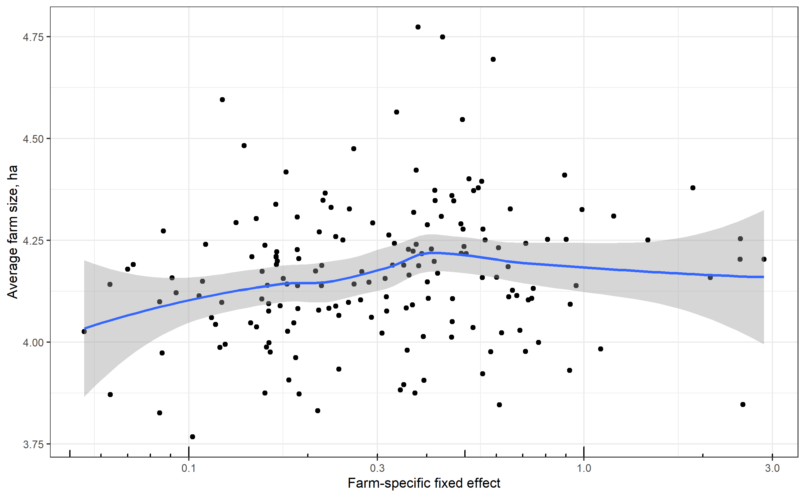
Let us compute average farm size and plot fixed effects versus farm size:

farm_mean_size <- farm_dta_log %>% group_by(id) %>% summarise(mean_size = mean(land))
glimpse(farm_mean_size)

Rows: 171
Columns: 2
$ id        <dbl> 101001, 101017, 101026, 101035, 101056, 101057, 101067, 1010…
$ mean_size <dbl> 2.5240000, 0.7230000, 0.1558333, 0.3211667, 0.3360000, 0.189…

plot_dta <- farm_mean_size %>% left_join(fef_dta)
glimpse(plot_dta)

Rows: 171
Columns: 6
$ id           <dbl> 101001, 101017, 101026, 101035, 101056, 101057, 101067, 1…
$ mean_size    <dbl> 2.5240000, 0.7230000, 0.1558333, 0.3211667, 0.3360000, 0.…
$ Estimate     <dbl> 3.847036, 4.103960, 4.237548, 4.263063, 4.564856, 4.20514…
$ `Std. Error` <dbl> 0.3166160, 0.2819603, 0.2847204, 0.2792276, 0.2846006, 0.…
$ `t-value`    <dbl> 12.15048, 14.55510, 14.88319, 15.26734, 16.03951, 14.3927…
$ `Pr(>|t|)`   <dbl> 1.958956e-31, 5.202280e-43, 1.090622e-44, 1.109427e-46, 9…

plot_dta %>% ggplot() + aes(x = mean_size, y = Estimate) + 
  geom_point() + geom_smooth() + scale_x_log10() +
  xlab("Farm-specific fixed effect") + 
  ylab("Average farm size, ha") + 
  annotation_logticks(side = "b")

Farm size and efficiency

References

Battese, G. E. (1997). A note on the estimation of cobb-douglas production functions when some explanatory variables have zero values. Journal of Agricultural Economics, 48(1-3), 250–252. http://doi.org/10.1111/j.1477-9552.1997.tb01149.x

Panel Regression Analysis: Micro application to production function

Example 2. Micro-level application of panel regression analysis RiceFarms

Part 1. Theoretical basis

Estimation strategy. Part 1.

What about OVB?

Using the OVB formula

How to resolve such OVB?

Estimation strategy. Part 2.

Estimation strategy. Part 3. Return to scale (1)

Estimation strategy. Part 3. Return to scale (2)

Estimation strategy. Part 3. Return to scale (3)

Part 2. Exploratory data analysis and data description

Data preparation

Computing yields and logs

Summary statistics

Any problems with data?

-Infinity in logs: lazy solution

-Infinity in logs: smart solution

Summary statistics after data cleaning

Farm size vs rice yields

Farm size vs rice yields

Farm size vs rice yields by year

Part 3. Estimating the models

Step 1 Pooled OLS

Step 1 Linearity and homoscedasticity

Step 1 Collinearity

Step 2 Fixed Effect

Step 2 FE with lazy log(0)

Step 2.2 F test for individual effects

Step 2.3 Lagrange Multiplier Tests

Step 2 Random Effect

Step 2 Hausman Test for Panel Models

Step 3 Serial correlation and cross-sectional dependence

Step 3 lm tests for random effects and/or serial correlation

Step 4. Robust inference

Step 4. Robust inference

Step 4. Robust inference

Part 4. Return to scale (1)

Part 4. Return to scale (2)

Conclusions

Individual fixed effects

Extra on fixed effects

Individual fixed effects (extraction 1)

Individual fixed effects (extraction 3)

Farm size and efficiency

Farm size and efficiency

References

Example 2. Micro-level application of panel regression analysis `RiceFarms`

`-Infinity` in logs: lazy solution

`-Infinity` in logs: smart solution