Panel Regression Analysis
Eduard Bukin
Recap
Ceteris paribus!?
- Why multiple regression is “good”?
- What variables are important when establishing a causal effect of a treatment (key variable)?
- What if we do not have an important variable?
Selection bias = OVB! In multiple regression analysis.
- What does OVB to our regression estimates?
- Bias (inconsistency) of estimates!
Simpson’s paradox
See: Simpson, E. H. (1951). The Interpretation of Interaction in Contingency Tables. Journal of the Royal Statistical Society: Series B (Methodological), 13(2), 238–241. https://doi.org/10.1111/j.2517-6161.1951.tb00088.x
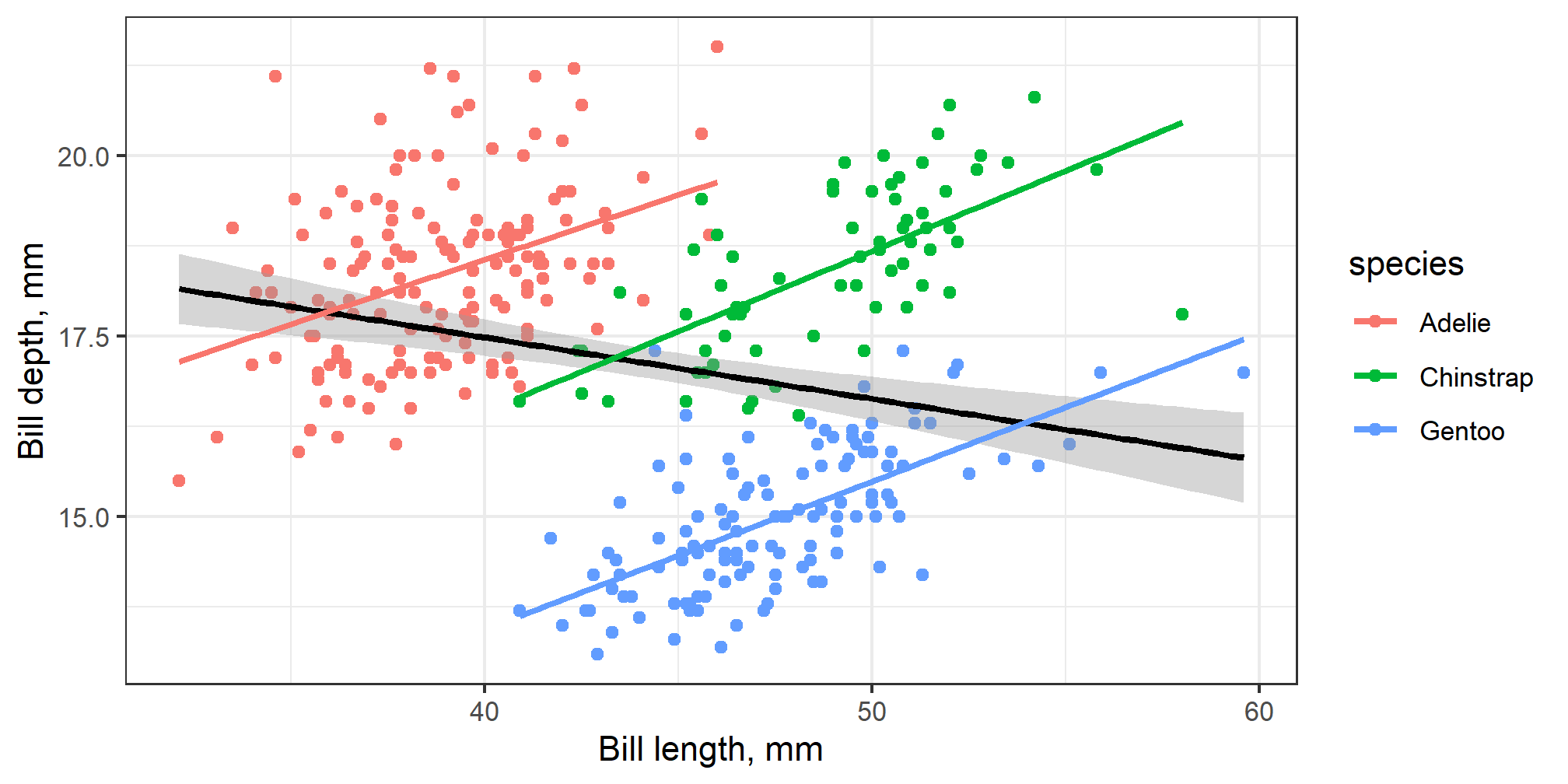
Simpson’s paradox (with penguins)
Let us investigate…
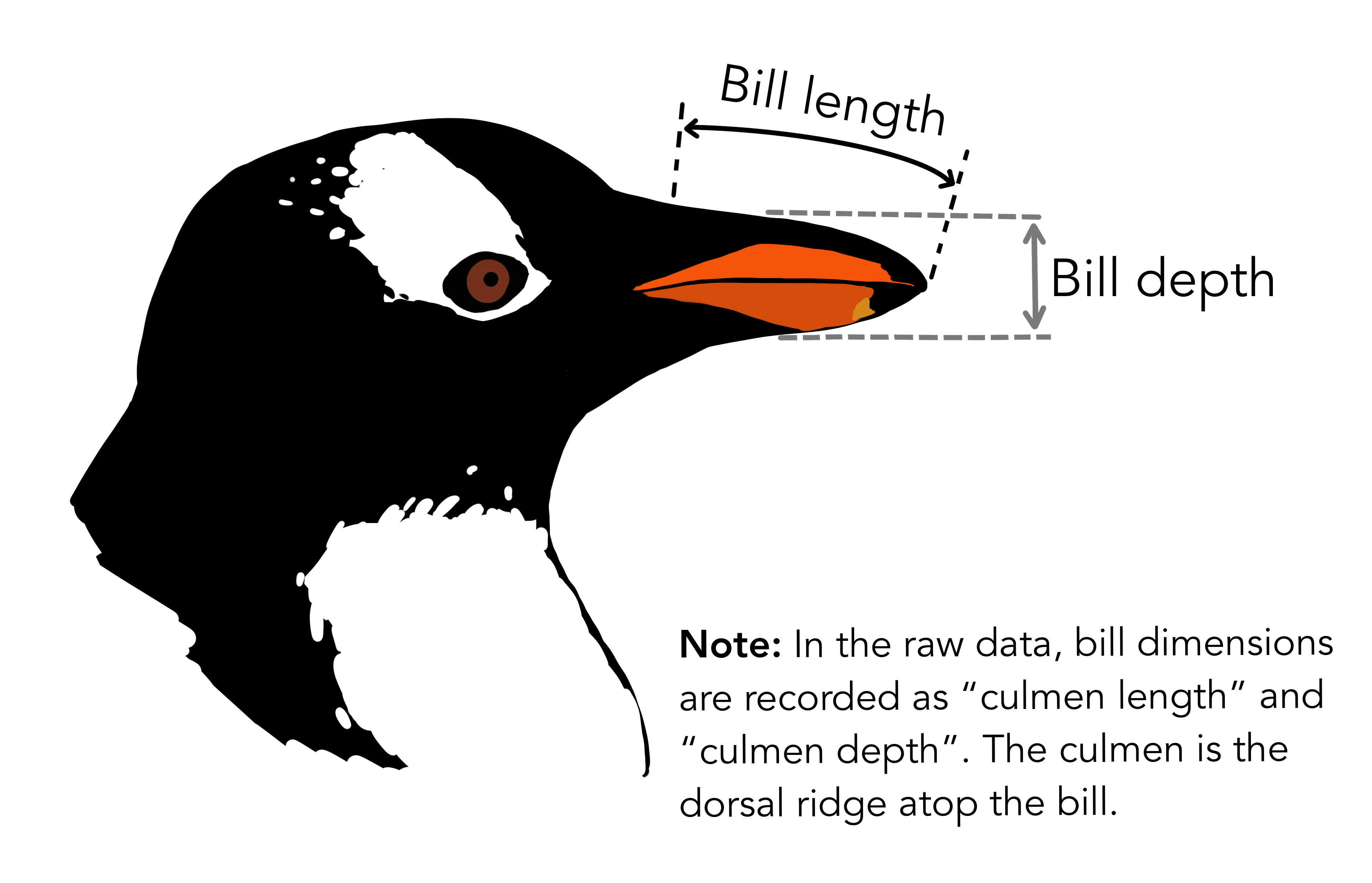
The relationship between bill length and depth in penguins…
The data
Rows: 344
Columns: 8
$ species           <fct> Adelie, Adelie, Adelie, Adelie, Adelie, Adelie, Adel…
$ island            <fct> Torgersen, Torgersen, Torgersen, Torgersen, Torgerse…
$ bill_length_mm    <dbl> 39.1, 39.5, 40.3, NA, 36.7, 39.3, 38.9, 39.2, 34.1, …
$ bill_depth_mm     <dbl> 18.7, 17.4, 18.0, NA, 19.3, 20.6, 17.8, 19.6, 18.1, …
$ flipper_length_mm <int> 181, 186, 195, NA, 193, 190, 181, 195, 193, 190, 186…
$ body_mass_g       <int> 3750, 3800, 3250, NA, 3450, 3650, 3625, 4675, 3475, …
$ sex               <fct> male, female, female, NA, female, male, female, male…
$ year              <int> 2007, 2007, 2007, 2007, 2007, 2007, 2007, 2007, 2007…
The relationship
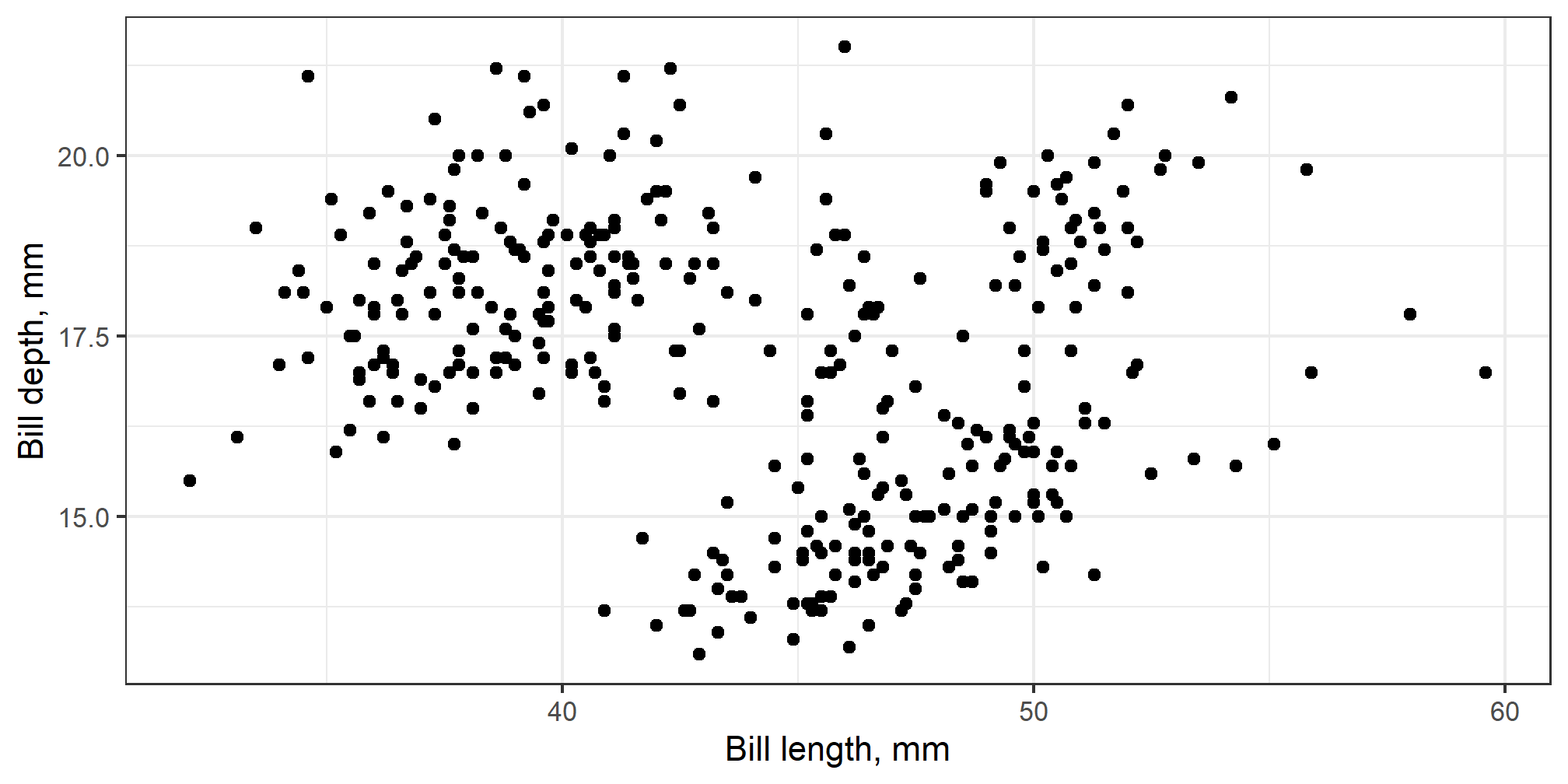
The trend
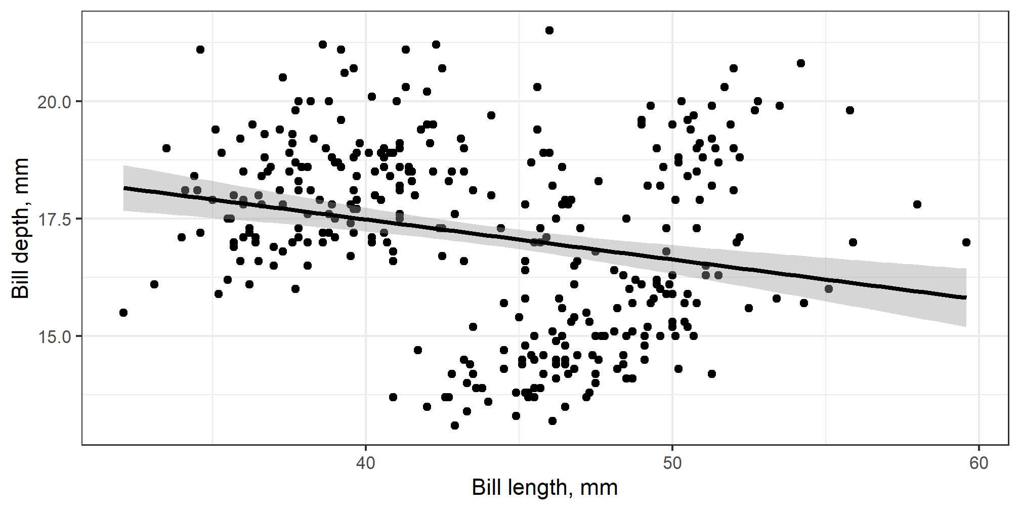
Is this the true trend?
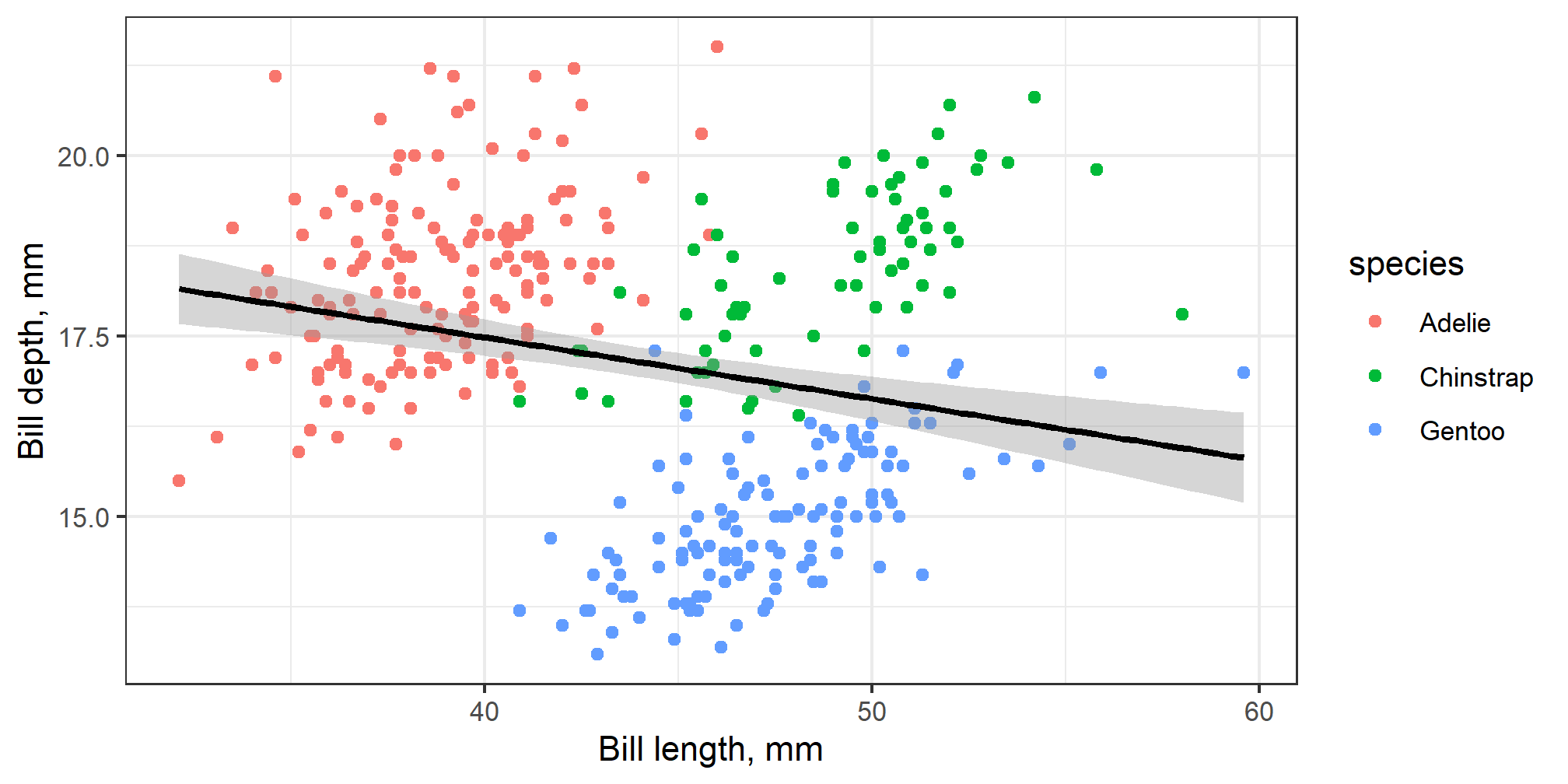
The true trends
Regression results
fit1 <- lm(bill_depth_mm ~ bill_length_mm, data = penguins)
fit2 <- lm(bill_depth_mm ~ bill_length_mm + species, data = penguins)
fit3 <- lm(bill_depth_mm ~ -1 + bill_length_mm + species, data = penguins)
modelsummary(
  list(fit1, fit2, fit3),
  estimate = "{estimate}{stars} ({std.error})",
  statistic = NULL,
  gof_map = c("nobs", "adj.r.squared")
)| (1) | (2) | (3) | |
|---|---|---|---|
| (Intercept) | 20.885*** (0.844) | 10.592*** (0.683) | |
| bill_length_mm | −0.085*** (0.019) | 0.200*** (0.017) | 0.200*** (0.017) |
| speciesChinstrap | −1.933*** (0.224) | 8.659*** (0.862) | |
| speciesGentoo | −5.106*** (0.191) | 5.486*** (0.835) | |
| speciesAdelie | 10.592*** (0.683) | ||
| Num.Obs. | 342 | 342 | 342 |
| R2 Adj. | 0.052 | 0.767 | 0.997 |
Simpson’s paradox conclusion
Trends or relationships are observed in the whole population, but they reverse or disappear, when each group is treated separately.
Causes:
Unobserved heterogeneity/differences between groups.
Underlining processes that are different between parts of the population.
Resolutions to the paradox:
Control variables in the MRL.
Panel data.
Data Types
Cross-sectional data
| ID | Y | X1 | X2 |
|---|---|---|---|
| \(1\) | \(y_{1}\) | \(x^{1}_{1}\) | \(x^{2}_{1}\) |
| \(2\) | \(y_{2}\) | \(x^{1}_{2}\) | \(x^{2}_{2}\) |
| \(3\) | \(y_{3}\) | \(x^{1}_{3}\) | \(x^{2}_{3}\) |
| \(4\) | \(y_{4}\) | \(x^{1}_{4}\) | \(x^{2}_{4}\) |
| \(5\) | \(y_{5}\) | \(x^{1}_{5}\) | \(x^{2}_{5}\) |
| \(6\) | \(y_{6}\) | \(x^{1}_{6}\) | \(x^{2}_{6}\) |
| \(\vdots\) | \(\vdots\) | \(\vdots\) | \(\vdots\) |
| \(N\) | \(y_{N}\) | \(x^{1}_{N}\) | \(x^{2}_{N}\) |
Data that we usually collect in a single data collection.
- Each individual is represented by one observation.
Could be repeatedly collected multiple times (repeated cross-section),
- but, in every repetition, there are different individuals!
Panel data
| ID | Time | Y | X1 | X2 |
|---|---|---|---|---|
| \(1\) | \(1\) | \(y_{11}\) | \(x^{1}_{11}\) | \(x^{2}_{11}\) |
| \(1\) | \(2\) | \(y_{12}\) | \(x^{1}_{12}\) | \(x^{2}_{12}\) |
| \(1\) | \(3\) | \(y_{13}\) | \(x^{1}_{13}\) | \(x^{2}_{13}\) |
| \(2\) | \(2\) | \(y_{22}\) | \(x^{1}_{22}\) | \(x^{2}_{22}\) |
| \(2\) | \(3\) | \(y_{23}\) | \(x^{1}_{23}\) | \(x^{2}_{23}\) |
| \(3\) | \(1\) | \(y_{31}\) | \(x^{1}_{31}\) | \(x^{2}_{31}\) |
| \(3\) | \(2\) | \(y_{32}\) | \(x^{1}_{32}\) | \(x^{2}_{32}\) |
| \(\vdots\) | \(\vdots\) | \(\vdots\) | \(\vdots\) | \(\vdots\) |
| \(N\) | \(1\) | \(y_{N1}\) | \(x^{1}_{N1}\) | \(x^{1}_{N1}\) |
| \(\vdots\) | \(\vdots\) | \(\vdots\) | \(\vdots\) | \(\vdots\) |
| \(N\) | \(T\) | \(y_{NT}\) | \(x^{1}_{NT}\) | \(x^{2}_{NT}\) |
table with data, where
each individual (cohort, e.i. region, country)
is represented by multiple observations at different time periods.
Panel data: Balanced and Unbalanced
Balanced
Each individual is represented in all time periods.
| \(\text{ID}\) | \(\text{Time}\) | \(Y\) | \(X\) |
|---|---|---|---|
| 1 | 1 | \(Y_{11}\) | \(X_{11}\) |
| 1 | 2 | \(Y_{12}\) | \(X_{12}\) |
| \(\vdots\) | \(\vdots\) | \(\vdots\) | \(\vdots\) |
| 1 | \(T\) | \(Y_{1T}\) | \(X_{1T}\) |
| 2 | 1 | \(Y_{21}\) | \(X_{21}\) |
| 2 | 2 | \(Y_{22}\) | \(X_{22}\) |
| \(\vdots\) | \(\vdots\) | \(\vdots\) | \(\vdots\) |
| 2 | \(T\) | \(Y_{2T}\) | \(X_{2T}\) |
| 3 | 1 | \(Y_{31}\) | \(X_{31}\) |
| \(\vdots\) | \(\vdots\) | \(\vdots\) | \(\vdots\) |
| \(N\) | \(T\) | \(Y_{NT}\) | \(X_{NT}\) |
Un balanced
Each individual only appears in some time periods (not all).
| \(\text{ID}\) | \(\text{Time}\) | \(Y\) | \(X\) |
|---|---|---|---|
| 1 | 1 | \(Y_{11}\) | \(X_{11}\) |
| 1 | 2 | \(Y_{12}\) | \(X_{12}\) |
| 2 | 2 | \(Y_{22}\) | \(X_{22}\) |
| 2 | 3 | \(Y_{23}\) | \(X_{23}\) |
| 3 | 3 | \(Y_{33}\) | \(X_{33}\) |
| 4 | 1 | \(Y_{41}\) | \(X_{41}\) |
| 5 | 2 | \(Y_{52}\) | \(X_{52}\) |
| \(\vdots\) | \(\vdots\) | \(\vdots\) | \(\vdots\) |
| \(N\) | \(T\) | \(Y_{NT}\) | \(X_{NT}\) |
Regressions with Panel Data
Important
is a strategy to control for unobserved/omitted but fixed heterogeneity using time or cohort (individual) dimensions.
There are:
Pooled regression
Least-squares dummy variable (LSDV) model
Fixed Effect Panel Regression (within, first-difference and between)
Random Effect Panel Regression
Example 1: Effect of an employee’s union membership on wage
Problem setting
Does the collective bargaining (union membership) has any effect on wages?
- See: (Card, 1996; Freeman, 1984)
\[ log(\text{Wage}_{it}) = \beta_0 + \beta_1 \cdot \text{Union}_{it} + \beta_2 \cdot {X_{it}} + \beta_3 \cdot \text{Ability}_{i} + \epsilon_{it} \]
where \(i\) is the individual and \(t\) is the time dimension;
Is there an endogeneity problem?
\[ log(\text{Wage}_{it}) = \beta_0 + \beta_1 \cdot \text{Union}_{it} + \beta_2 \cdot {X_{it}} + \beta_3 \cdot \text{Ability}_{i} + \epsilon_{it} \]
Is there a source of endogeneity / selection bias here?
- Any ideas?
\(\text{Ability}_{i}\) not observable and not measurable;
- time invariant;
- correlates with \(X\) and \(Y\);
Omitting ability causes bias
One of the solutions:
Ability are time-invariant and unique to each individual;
If we have multiple observation per each individual (panel data),
we can introduce dummy variables for each individual, to approximate ability.
This is also called Fixed Effect - regression model
or a within transformation model
or Difference in Difference
Other solutions:
Any ideas?
Introduce control variables that are proxy of ability.
Employ specific research design:
RCT
RDD
Empirical example
Rows: 4,165
Columns: 15
$ id      <dbl> 1, 1, 1, 1, 1, 1, 1, 2, 2, 2, 2, 2, 2, 2, 3, 3, 3, 3, 3, 3, 3,…
$ year    <dbl> 82, 83, 84, 85, 86, 87, 88, 82, 83, 84, 85, 86, 87, 88, 82, 83…
$ exper   <dbl> 3, 4, 5, 6, 7, 8, 9, 30, 31, 32, 33, 34, 35, 36, 6, 7, 8, 9, 1…
$ hours   <dbl> 32, 43, 40, 39, 42, 35, 32, 34, 27, 33, 30, 30, 37, 30, 50, 51…
$ bluecol <chr> "no", "no", "no", "no", "no", "no", "no", "yes", "yes", "yes",…
$ ind     <dbl> 0, 0, 0, 0, 1, 1, 1, 0, 0, 1, 1, 1, 1, 1, 1, 1, 1, 1, 1, 1, 1,…
$ south   <chr> "yes", "yes", "yes", "yes", "yes", "yes", "yes", "no", "no", "…
$ smsa    <chr> "no", "no", "no", "no", "no", "no", "no", "no", "no", "no", "n…
$ married <chr> "yes", "yes", "yes", "yes", "yes", "yes", "yes", "yes", "yes",…
$ union   <dbl> 0, 0, 0, 0, 0, 0, 0, 0, 0, 1, 0, 0, 0, 0, 1, 1, 1, 1, 1, 1, 1,…
$ educ    <dbl> 9, 9, 9, 9, 9, 9, 9, 11, 11, 11, 11, 11, 11, 11, 12, 12, 12, 1…
$ black   <chr> "no", "no", "no", "no", "no", "no", "no", "no", "no", "no", "n…
$ lwage   <dbl> 5.56068, 5.72031, 5.99645, 5.99645, 6.06146, 6.17379, 6.24417,…
$ female  <dbl> 1, 1, 1, 1, 1, 1, 1, 1, 1, 1, 1, 1, 1, 1, 1, 1, 1, 1, 1, 1, 1,…
$ wage    <dbl> 259.9996, 304.9995, 401.9992, 401.9992, 429.0013, 480.0019, 51…
The data
| id | year | exper | hours | bluecol | ind | south | smsa | married | union | educ | black | lwage | female | wage |
|---|---|---|---|---|---|---|---|---|---|---|---|---|---|---|
| 5 | 82 | 10 | 50 | yes | 0 | no | no | yes | 1 | 16 | no | 6.43775 | 1 | 624.9990 |
| 5 | 83 | 11 | 46 | yes | 0 | no | no | yes | 1 | 16 | no | 6.62007 | 1 | 749.9976 |
| 5 | 84 | 12 | 40 | yes | 0 | no | no | yes | 1 | 16 | no | 6.63332 | 1 | 760.0012 |
| 5 | 85 | 13 | 50 | no | 0 | no | no | yes | 0 | 16 | no | 6.98286 | 1 | 1077.9970 |
| 5 | 86 | 14 | 47 | yes | 0 | no | yes | yes | 0 | 16 | no | 7.04752 | 1 | 1150.0032 |
| 5 | 87 | 15 | 47 | no | 0 | no | no | yes | 0 | 16 | no | 7.31322 | 1 | 1499.9994 |
| 5 | 88 | 16 | 49 | no | 0 | no | no | yes | 0 | 16 | no | 7.29574 | 1 | 1474.0073 |
| 168 | 82 | 3 | 40 | no | 0 | no | yes | yes | 0 | 17 | no | 6.23245 | 1 | 509.0010 |
| 168 | 83 | 4 | 42 | no | 0 | no | yes | yes | 0 | 17 | no | 6.57925 | 1 | 719.9991 |
| 168 | 84 | 5 | 44 | no | 0 | no | yes | yes | 1 | 17 | no | 6.65286 | 1 | 774.9977 |
| 168 | 85 | 6 | 48 | no | 0 | no | yes | yes | 1 | 17 | no | 6.74524 | 1 | 850.0031 |
| 168 | 86 | 7 | 48 | no | 0 | no | yes | yes | 0 | 17 | no | 7.49554 | 1 | 1799.9965 |
| 168 | 87 | 8 | 48 | no | 0 | no | yes | yes | 0 | 17 | no | 8.16052 | 1 | 3500.0061 |
| 168 | 88 | 9 | 50 | no | 0 | no | yes | yes | 0 | 17 | no | 8.30820 | 1 | 4057.0038 |
Pooled Regression
\[ log(\text{Wage}_{it}) = \beta_0 + \beta_1 \cdot \text{Union}_{it} + \beta_2 \cdot {X_{it}} + \epsilon_{it} \]
- Regression model on all observations in the panel data set without any individual effects.
Call:
lm(formula = log(wage) ~ union + educ + exper + I(exper^2) +
    hours, data = wage_dta)

Coefficients:
(Intercept)        union         educ        exper   I(exper^2)        hours
  4.7054380    0.1261467    0.0819744    0.0437155   -0.0006932    0.0077042
Least-squares dummy variable (LSDV)
\[ log(\text{Wage}_{it}) = \beta_0 + \beta_1 \cdot \text{Union}_{it} + \beta_2 \cdot {X_{it}} + \beta_3 \cdot \color{Red}{\delta_{i}} + \epsilon_{it} \]
Pooled regression plus dummy variable for each individual.
This is not a Fixed Effect Panel Regression!
Call:
lm(formula = log(wage) ~ union + educ + exper + I(exper^2) +
    hours + factor(id), data = wage_dta)

Coefficients:
  (Intercept)          union           educ          exper     I(exper^2)
    4.3485732      0.0300295      0.1023231      0.1137052     -0.0004234
        hours    factor(id)2    factor(id)3    factor(id)4    factor(id)5
    0.0007980     -2.2946317     -0.1234092     -2.3978310     -0.5366805
  factor(id)6    factor(id)7    factor(id)8    factor(id)9   factor(id)10
   -1.4597761     -1.2411420     -1.5180049      0.2078530     -0.1734390
 factor(id)11   factor(id)12   factor(id)13   factor(id)14   factor(id)15
   -1.4704689     -1.3608691     -1.3890339     -1.0439450     -0.9439428
 factor(id)16   factor(id)17   factor(id)18   factor(id)19   factor(id)20
   -1.5809655     -0.9700846     -1.3922150     -3.0892451     -1.8367302
 factor(id)21   factor(id)22   factor(id)23   factor(id)24   factor(id)25
   -1.7226414     -1.4223248      0.0054199     -0.8357823     -0.6064977
 factor(id)26   factor(id)27   factor(id)28   factor(id)29   factor(id)30
   -0.7379286     -0.2772751     -1.8216457     -1.8871665     -1.3042601
 factor(id)31   factor(id)32   factor(id)33   factor(id)34   factor(id)35
   -1.4134898     -1.8734643     -0.6413820     -3.7105381     -0.1984895
 factor(id)36   factor(id)37   factor(id)38   factor(id)39   factor(id)40
   -0.3421001     -0.3410200     -0.7597065     -0.0688068     -1.7787978
 factor(id)41   factor(id)42   factor(id)43   factor(id)44   factor(id)45
   -1.0532843     -2.2573678      0.1550164      0.0478652     -0.9543507
 factor(id)46   factor(id)47   factor(id)48   factor(id)49   factor(id)50
   -0.2541933     -1.7069053     -1.8137723     -1.9258846     -2.4484643
 factor(id)51   factor(id)52   factor(id)53   factor(id)54   factor(id)55
   -1.9760363     -1.6064527     -0.4646712     -0.4521180     -1.7422486
 factor(id)56   factor(id)57   factor(id)58   factor(id)59   factor(id)60
   -1.9282946     -1.6643194     -2.8323912     -1.7329928     -1.6527519
 factor(id)61   factor(id)62   factor(id)63   factor(id)64   factor(id)65
   -1.9914748     -0.1579195     -0.2806420     -2.6926172     -1.7074951
 factor(id)66   factor(id)67   factor(id)68   factor(id)69   factor(id)70
   -1.0021172     -2.5046091     -2.5941980     -2.0777134     -0.4562135
 factor(id)71   factor(id)72   factor(id)73   factor(id)74   factor(id)75
   -0.0984012     -0.9192300     -0.9709685     -0.7050966     -1.7193154
 factor(id)76   factor(id)77   factor(id)78   factor(id)79   factor(id)80
   -1.1672133     -0.7934024     -3.4592869     -0.8823052     -0.0604197
 factor(id)81   factor(id)82   factor(id)83   factor(id)84   factor(id)85
   -0.2728831     -1.3694580     -0.8873794     -3.4094508     -0.6181149
 factor(id)86   factor(id)87   factor(id)88   factor(id)89   factor(id)90
    0.3230099     -0.6208690     -0.0384965     -0.7156531      0.2819298
 factor(id)91   factor(id)92   factor(id)93   factor(id)94   factor(id)95
    0.2219382     -0.0389122     -2.2703900     -0.6713527     -2.5658913
 factor(id)96   factor(id)97   factor(id)98   factor(id)99  factor(id)100
   -1.8929945     -2.3668088     -1.0815051     -1.2371669     -0.3689453
factor(id)101  factor(id)102  factor(id)103  factor(id)104  factor(id)105
   -2.0715701      0.2419079     -1.0534000     -1.2417073     -0.3892415
factor(id)106  factor(id)107  factor(id)108  factor(id)109  factor(id)110
    0.0013452     -1.8143890     -0.9852634     -1.4033012     -2.7813619
factor(id)111  factor(id)112  factor(id)113  factor(id)114  factor(id)115
   -0.1122968     -0.8453668     -1.8469750     -2.9350313     -0.4420842
factor(id)116  factor(id)117  factor(id)118  factor(id)119  factor(id)120
   -0.7258607     -1.2304082     -1.3950810     -0.3204476     -0.7104122
factor(id)121  factor(id)122  factor(id)123  factor(id)124  factor(id)125
   -0.3685394     -0.6871320     -1.5356558     -1.9044675     -0.9214093
factor(id)126  factor(id)127  factor(id)128  factor(id)129  factor(id)130
    0.1863200     -1.8088881     -2.3404805     -2.3327080     -1.8672439
factor(id)131  factor(id)132  factor(id)133  factor(id)134  factor(id)135
   -1.7733156     -1.2515247     -1.2618072     -0.2715418     -0.5405965
factor(id)136  factor(id)137  factor(id)138  factor(id)139  factor(id)140
   -0.9040781     -1.2464677     -1.3348897      0.0546240     -0.1468334
factor(id)141  factor(id)142  factor(id)143  factor(id)144  factor(id)145
   -0.9653104     -2.8803152     -2.5587496     -0.3057205     -1.1895399
factor(id)146  factor(id)147  factor(id)148  factor(id)149  factor(id)150
   -2.5564297     -0.3336869     -0.2135711     -0.2358201     -0.9902041
factor(id)151  factor(id)152  factor(id)153  factor(id)154  factor(id)155
   -1.8371688     -0.3919091     -0.9059245     -0.8288426      0.2639585
factor(id)156  factor(id)157  factor(id)158  factor(id)159  factor(id)160
   -2.3669688     -0.1579770     -1.9607783     -2.2903756     -2.0867318
factor(id)161  factor(id)162  factor(id)163  factor(id)164  factor(id)165
   -0.4052899     -0.5879060     -0.7129091     -0.5237673     -3.0691480
factor(id)166  factor(id)167  factor(id)168  factor(id)169  factor(id)170
   -0.3346194     -1.2951818      0.3693013     -1.6563817     -2.1460479
factor(id)171  factor(id)172  factor(id)173  factor(id)174  factor(id)175
   -1.0321605     -0.2130777     -1.7902925      0.1377581     -0.0160055
factor(id)176  factor(id)177  factor(id)178  factor(id)179  factor(id)180
    0.2569786     -1.6326400      0.4028510     -2.3587711     -0.3845946
factor(id)181  factor(id)182  factor(id)183  factor(id)184  factor(id)185
   -0.4108327     -0.9834346     -1.0972550     -1.6781968     -1.5026082
factor(id)186  factor(id)187  factor(id)188  factor(id)189  factor(id)190
   -2.1577766     -1.1647283     -0.1239156     -1.7815425      0.2619762
factor(id)191  factor(id)192  factor(id)193  factor(id)194  factor(id)195
   -1.4993833      0.0160729     -2.2211180     -0.4287428     -0.8272276
factor(id)196  factor(id)197  factor(id)198  factor(id)199  factor(id)200
    0.1178582     -1.5464632     -1.9258471     -0.1875497     -0.3310429
factor(id)201  factor(id)202  factor(id)203  factor(id)204  factor(id)205
   -1.4934470     -0.5369335     -1.5108323     -2.0658719     -1.6709767
factor(id)206  factor(id)207  factor(id)208  factor(id)209  factor(id)210
   -0.0090120     -0.5221725     -1.6804807     -2.0796591     -2.0767268
factor(id)211  factor(id)212  factor(id)213  factor(id)214  factor(id)215
   -1.4748328     -0.0448817     -1.4898530     -1.9329652     -3.5076699
factor(id)216  factor(id)217  factor(id)218  factor(id)219  factor(id)220
   -1.1255642     -0.2327264     -0.6513809     -0.8178650     -2.4156438
factor(id)221  factor(id)222  factor(id)223  factor(id)224  factor(id)225
   -2.1017309      0.0331950     -1.0231728     -1.4645738     -0.5458016
factor(id)226  factor(id)227  factor(id)228  factor(id)229  factor(id)230
   -3.0261551     -2.2929047      0.2832356     -1.3169281      0.2964316
factor(id)231  factor(id)232  factor(id)233  factor(id)234  factor(id)235
   -1.0946220     -2.2743788     -1.8237789     -1.6554734     -1.2081230
factor(id)236  factor(id)237  factor(id)238  factor(id)239  factor(id)240
   -0.0145449     -0.6384647     -2.1569987     -1.4416687     -2.0393688
factor(id)241  factor(id)242  factor(id)243  factor(id)244  factor(id)245
   -0.5874512     -0.5934676      0.2367489     -1.4340693     -2.3045132
factor(id)246  factor(id)247  factor(id)248  factor(id)249  factor(id)250
   -2.7880182     -0.7003395     -1.1107962     -2.4985511     -1.3364049
factor(id)251  factor(id)252  factor(id)253  factor(id)254  factor(id)255
   -0.6067969     -1.5576645     -0.0986338     -2.6540530      0.0383125
factor(id)256  factor(id)257  factor(id)258  factor(id)259  factor(id)260
   -0.2349775     -2.1928398     -2.3075449     -0.7143545     -0.1095476
factor(id)261  factor(id)262  factor(id)263  factor(id)264  factor(id)265
   -0.7968060     -0.5774167     -0.6080097     -0.1404218     -0.6091514
factor(id)266  factor(id)267  factor(id)268  factor(id)269  factor(id)270
   -1.5381684     -0.6415396     -0.8257309     -0.9420411     -0.8422041
factor(id)271  factor(id)272  factor(id)273  factor(id)274  factor(id)275
   -0.4524016     -0.2456966     -1.7472768     -1.0506405     -0.0310502
factor(id)276  factor(id)277  factor(id)278  factor(id)279  factor(id)280
    0.3472376     -2.0224341      0.1895913     -0.6614986     -2.7705095
factor(id)281  factor(id)282  factor(id)283  factor(id)284  factor(id)285
    0.2245524     -1.3899214     -2.7102791     -2.2411764      0.2478444
factor(id)286  factor(id)287  factor(id)288  factor(id)289  factor(id)290
   -0.3704373     -0.5927907     -0.2396347     -1.6533998     -0.0958892
factor(id)291  factor(id)292  factor(id)293  factor(id)294  factor(id)295
   -2.5107176     -1.7989286     -0.5703390     -1.2011109     -1.4576638
factor(id)296  factor(id)297  factor(id)298  factor(id)299  factor(id)300
   -1.9986368     -0.5870901     -0.7176117     -3.2822239     -2.7838597
factor(id)301  factor(id)302  factor(id)303  factor(id)304  factor(id)305
   -0.3324034     -1.0640144      0.2979783     -0.4636494     -1.1197335
factor(id)306  factor(id)307  factor(id)308  factor(id)309  factor(id)310
   -1.2954014      0.8212389     -1.8036660     -1.3745703     -0.7606135
factor(id)311  factor(id)312  factor(id)313  factor(id)314  factor(id)315
    0.2105132     -0.8752712     -0.6629730     -0.4802000     -1.0600291
factor(id)316  factor(id)317  factor(id)318  factor(id)319  factor(id)320
   -1.9089897     -0.9238980     -0.6972992     -1.6439082     -0.9770545
factor(id)321  factor(id)322  factor(id)323  factor(id)324  factor(id)325
   -0.2597240     -0.3929224     -0.8099876      0.2160266     -3.1693716
factor(id)326  factor(id)327  factor(id)328  factor(id)329  factor(id)330
   -1.3707289     -0.8099548     -1.9741880     -3.2232714     -2.9081193
factor(id)331  factor(id)332  factor(id)333  factor(id)334  factor(id)335
   -2.4720627     -3.4967480      0.0880504     -2.4198878     -2.0780789
factor(id)336  factor(id)337  factor(id)338  factor(id)339  factor(id)340
   -2.3475630      0.5764727     -0.6084878     -0.8872653     -1.9636734
factor(id)341  factor(id)342  factor(id)343  factor(id)344  factor(id)345
    0.0883837     -1.8502495     -1.4848842     -0.9710595     -1.2319603
factor(id)346  factor(id)347  factor(id)348  factor(id)349  factor(id)350
   -1.7024146     -1.3434399     -1.3863174      0.4956454     -2.5654191
factor(id)351  factor(id)352  factor(id)353  factor(id)354  factor(id)355
   -1.3784243      0.0816134     -1.7059876     -1.3627206     -0.4565893
factor(id)356  factor(id)357  factor(id)358  factor(id)359  factor(id)360
    0.3603776     -0.9685689     -1.3991295     -3.0412550     -1.6851473
factor(id)361  factor(id)362  factor(id)363  factor(id)364  factor(id)365
   -0.7058692     -0.9195798     -1.0953487     -1.4769641     -2.6742985
factor(id)366  factor(id)367  factor(id)368  factor(id)369  factor(id)370
   -0.6578946     -1.2999971     -0.3382028      0.3863243     -0.0720030
factor(id)371  factor(id)372  factor(id)373  factor(id)374  factor(id)375
   -1.9432209     -0.6223422     -1.1822873     -0.9548354     -2.0004202
factor(id)376  factor(id)377  factor(id)378  factor(id)379  factor(id)380
   -1.9659526     -1.0630786      0.2863626     -0.9885524     -2.2528915
factor(id)381  factor(id)382  factor(id)383  factor(id)384  factor(id)385
   -1.8595097     -1.5724380     -1.8713639     -2.5344664     -0.1624537
factor(id)386  factor(id)387  factor(id)388  factor(id)389  factor(id)390
   -0.6421035     -0.3629400     -2.3279087     -1.1232122     -1.7657519
factor(id)391  factor(id)392  factor(id)393  factor(id)394  factor(id)395
   -2.5207200     -1.6091356     -0.8136357      0.2210733     -2.2452954
factor(id)396  factor(id)397  factor(id)398  factor(id)399  factor(id)400
   -0.6756564      0.1621353     -0.8481867     -1.7341285     -0.3817257
factor(id)401  factor(id)402  factor(id)403  factor(id)404  factor(id)405
    0.2949123     -0.8927519     -0.9338798     -0.7166768      0.3456415
factor(id)406  factor(id)407  factor(id)408  factor(id)409  factor(id)410
    0.2419052     -1.8216061     -0.4228484     -2.9393318     -2.0225911
factor(id)411  factor(id)412  factor(id)413  factor(id)414  factor(id)415
   -0.4310985      0.4951506     -0.3954707     -2.8343863     -1.6226128
factor(id)416  factor(id)417  factor(id)418  factor(id)419  factor(id)420
   -2.2101251     -0.3836277     -2.0551281     -0.3642385     -0.4022928
factor(id)421  factor(id)422  factor(id)423  factor(id)424  factor(id)425
   -1.4834110     -0.5625562     -0.6107236      0.1691667      0.3211209
factor(id)426  factor(id)427  factor(id)428  factor(id)429  factor(id)430
    0.2279390     -1.8875790     -3.0841075     -0.6159943     -0.3415796
factor(id)431  factor(id)432  factor(id)433  factor(id)434  factor(id)435
   -0.7118149     -1.5641616     -1.9801839      0.1450722     -0.2017439
factor(id)436  factor(id)437  factor(id)438  factor(id)439  factor(id)440
   -0.3145338     -1.1190083     -1.7823379     -0.3957654     -0.9003941
factor(id)441  factor(id)442  factor(id)443  factor(id)444  factor(id)445
   -2.3437182     -3.4028128     -1.7003478      0.7524891     -1.0873692
factor(id)446  factor(id)447  factor(id)448  factor(id)449  factor(id)450
   -0.5228583     -1.8009627     -2.2900269     -0.2715184      0.1416728
factor(id)451  factor(id)452  factor(id)453  factor(id)454  factor(id)455
   -0.3214500     -0.7690325     -2.2657456     -0.0174455     -1.6515788
factor(id)456  factor(id)457  factor(id)458  factor(id)459  factor(id)460
   -1.4418559     -2.8946224     -0.9420793     -1.4296444      0.1185207
factor(id)461  factor(id)462  factor(id)463  factor(id)464  factor(id)465
   -2.2330238     -2.5544505     -0.9337258     -3.5688408     -0.2714708
factor(id)466  factor(id)467  factor(id)468  factor(id)469  factor(id)470
   -2.2471530     -1.8575604     -3.0165280     -4.3707337     -0.1020631
factor(id)471  factor(id)472  factor(id)473  factor(id)474  factor(id)475
   -2.2962452     -0.4362524     -0.0682312     -0.7113828     -0.6509739
factor(id)476  factor(id)477  factor(id)478  factor(id)479  factor(id)480
   -2.2159030     -0.3722269     -0.1277137     -0.8617902     -1.3784264
factor(id)481  factor(id)482  factor(id)483  factor(id)484  factor(id)485
   -1.2668125     -0.3221145     -0.3694822      0.3742597     -1.1971520
factor(id)486  factor(id)487  factor(id)488  factor(id)489  factor(id)490
   -1.7667638     -0.3340940     -1.7205133     -2.2568467     -1.8137394
factor(id)491  factor(id)492  factor(id)493  factor(id)494  factor(id)495
   -0.0582747     -1.9190715     -0.6342174     -3.6974693     -0.3921098
factor(id)496  factor(id)497  factor(id)498  factor(id)499  factor(id)500
   -1.5298775     -0.5476525     -1.4930554     -2.5228905     -0.2511241
factor(id)501  factor(id)502  factor(id)503  factor(id)504  factor(id)505
   -2.0783921     -1.0366267      0.3891613     -0.0326843     -1.4013691
factor(id)506  factor(id)507  factor(id)508  factor(id)509  factor(id)510
    0.1109218     -1.7455372     -2.6679473     -1.1284840      0.1729925
factor(id)511  factor(id)512  factor(id)513  factor(id)514  factor(id)515
   -0.8348753      0.4589049     -2.5682984     -0.9878010     -0.5940622
factor(id)516  factor(id)517  factor(id)518  factor(id)519  factor(id)520
   -1.7425469     -0.8692734     -1.1061395     -0.2754527     -2.0568223
factor(id)521  factor(id)522  factor(id)523  factor(id)524  factor(id)525
   -1.2248788      0.4854992      0.3539625     -0.4260779     -0.6468819
factor(id)526  factor(id)527  factor(id)528  factor(id)529  factor(id)530
   -0.0903952     -0.2045723     -0.4261753     -2.0586098     -0.1378354
factor(id)531  factor(id)532  factor(id)533  factor(id)534  factor(id)535
    0.5090071     -0.3524712     -2.7228941     -0.5025199     -1.0624910
factor(id)536  factor(id)537  factor(id)538  factor(id)539  factor(id)540
   -0.3035858     -0.4137570     -0.5286483      0.1598279     -1.4470984
factor(id)541  factor(id)542  factor(id)543  factor(id)544  factor(id)545
   -0.3111554     -1.0187912     -0.1758000      0.3356895     -2.5147919
factor(id)546  factor(id)547  factor(id)548  factor(id)549  factor(id)550
   -0.2690522      0.0699535     -0.3780972     -0.5916537     -0.1192377
factor(id)551  factor(id)552  factor(id)553  factor(id)554  factor(id)555
   -0.4489108     -0.5228657     -0.2531003     -1.4951698     -1.6801842
factor(id)556  factor(id)557  factor(id)558  factor(id)559  factor(id)560
    0.3760810     -1.0286751     -1.1760088     -3.2089989     -2.5710271
factor(id)561  factor(id)562  factor(id)563  factor(id)564  factor(id)565
    0.0315641      0.1818021     -2.2825744      0.0822954     -1.1950727
factor(id)566  factor(id)567  factor(id)568  factor(id)569  factor(id)570
    0.1940021     -3.5865482     -0.2442893     -1.0425527     -0.7318057
factor(id)571  factor(id)572  factor(id)573  factor(id)574  factor(id)575
   -0.0624118      0.0528832     -0.1803426      0.2557702     -0.6287755
factor(id)576  factor(id)577  factor(id)578  factor(id)579  factor(id)580
    0.2609783     -0.8120050     -0.0670469     -0.4403119      0.0559130
factor(id)581  factor(id)582  factor(id)583  factor(id)584  factor(id)585
   -0.3724249      0.3466553      0.1053244      0.0263852     -0.1070240
factor(id)586  factor(id)587  factor(id)588  factor(id)589  factor(id)590
   -1.3060257     -0.3438155     -0.2917004     -2.1209831      0.3472921
factor(id)591  factor(id)592  factor(id)593  factor(id)594  factor(id)595
   -2.2030413      0.0168668     -1.0857457     -0.0342374             NA
Data structure in the LSDV
| ID | Time | Y | X1 | X2 | \(\delta_1\) | \(\delta_2\) | \(\delta_N\) |
|---|---|---|---|---|---|---|---|
| \(1\) | \(1\) | \(y_{11}\) | \(x^{1}_{11}\) | \(x^{2}_{11}\) | 1 | 0 | 0 |
| \(1\) | \(2\) | \(y_{12}\) | \(x^{1}_{12}\) | \(x^{2}_{12}\) | 1 | 0 | 0 |
| \(1\) | \(3\) | \(y_{13}\) | \(x^{1}_{13}\) | \(x^{2}_{13}\) | 1 | 0 | 0 |
| \(2\) | \(2\) | \(y_{22}\) | \(x^{1}_{22}\) | \(x^{2}_{22}\) | 0 | 1 | 0 |
| \(2\) | \(3\) | \(y_{23}\) | \(x^{1}_{23}\) | \(x^{2}_{23}\) | 0 | 1 | 0 |
| \(\vdots\) | \(\vdots\) | \(\vdots\) | \(\vdots\) | \(\vdots\) | \(\vdots\) | \(\vdots\) | \(\vdots\) |
| \(N\) | \(1\) | \(y_{N1}\) | \(x^{1}_{N1}\) | \(x^{1}_{N1}\) | 0 | 0 | 1 |
| \(N\) | \(2\) | \(y_{N2}\) | \(x^{1}_{N2}\) | \(x^{2}_{N2}\) | 0 | 0 | 1 |
Results
modelsummary(
  list(
    `Pooled` = union_fit_0,
    `Least-squares dummy variable` = union_fit_1),
  estimate = "{estimate}{stars} ({std.error})",
  statistic = NULL,
  coef_map = c("(Intercept)", "union", "educ", "exper", "hours", "tenure"),
  gof_map = c("nobs", "adj.r.squared" , "df"),
  notes = "In the Least-squares dummy variable model we omitted all individual-related variables"
)| Pooled | Least-squares dummy variable | |
|---|---|---|
| (Intercept) | 4.705*** (0.070) | 4.349*** (0.289) |
| union | 0.126*** (0.013) | 0.030* (0.015) |
| educ | 0.082*** (0.002) | 0.102*** (0.027) |
| exper | 0.044*** (0.002) | 0.114*** (0.002) |
| hours | 0.008*** (0.001) | 0.001 (0.001) |
| Num.Obs. | 4165 | 4165 |
| R2 Adj. | 0.298 | 0.891 |
| DF | 5 | 598 |
| In the Least-squares dummy variable model we omitted all individual-related variables |
Cross-sectional data and LSDV (1)
Can we run a LSDV model with the cross-sectional data?
Any ideas?
Why?….
NO…
Because the number of independent variables have to be less then or equal to the number of observations.
Cross-sectional data and LSDV (2)
| ID | Y | X1 | X2 | \(\delta_1\) | \(\delta_2\) | \(\delta_3\) | \(\delta_N\) |
|---|---|---|---|---|---|---|---|
| \(1\) | \(y_{1}\) | \(x^{1}_{1}\) | \(x^{2}_{1}\) | 1 | 0 | 0 | 0 |
| \(2\) | \(y_{2}\) | \(x^{1}_{2}\) | \(x^{2}_{2}\) | 0 | 1 | 0 | 0 |
| \(3\) | \(y_{3}\) | \(x^{1}_{3}\) | \(x^{2}_{3}\) | 0 | 0 | 1 | 0 |
| \(\vdots\) | \(\vdots\) | \(\vdots\) | \(\vdots\) | \(\vdots\) | \(\vdots\) | \(\vdots\) | \(\vdots\) |
| \(N\) | \(y_{N}\) | \(x^{1}_{N}\) | \(x^{1}_{N}\) | 0 | 0 | 0 | 1 |
Panel data and LSDV
LSDV model works with the panel data, but…
it is inefficient! Any ideas why?…
Number of dummy variables is equal to the number of individuals + control variables.
- If we have 5,000 individuals, we have 5,000+ regression coefficients.
- What if we have 100,000 individuals?
Having too many regressors remains unbiased, but complicates inference:
- number of degrees of freedom increases;
- adjusted \(R^2\) may shrink to zero;
Panel regression: brief theory
Readings
Terminology
Panel data has:
- \(i\) individuals (groups);
- \(t\) time periods for each individual; and
- \(k\) independent variables \(x\)
Panel Regression could be:
Pooled OLS (regression without any panel structure);
Fixed Effect:
- Least-squares dummy variable (Pooled OLS + individual dummies);
- Within-transformation panel regression most commonly used
- First-difference, Between transformation panel regressions (look it up in (Croissant & Millo, 2018))
Random Effect panel regression
Pooled OLS
OLS regression on the entire data set with panel structure.
\[ y_{it} = \beta_0 + \beta_1 \cdot x_{1it} + \beta_2 \cdot x_{2it} + \dots + \beta_k \cdot x_{kit} + \epsilon_{it} \]
Estimates are biased because of the OVB.
We assume the OVB to be time-invariant.
Least-squares dummy variable model
\[ y_{it} = \beta_0 + \beta_1 \cdot x_{1it} + \beta_2 \cdot x_{2it} + \dots + \beta_k \cdot x_{kit} + \gamma_i \cdot \color{Red}{\delta_{i}} + \epsilon_{it} \]
Introduces a vector of dummy variables \(\color{Red}{\delta}\) and estimated coefficients \(\gamma_i\) for each dummy variable.
Estimates \(\hat \beta\) and \(\hat \gamma\) are unbiased (consistent) but inefficient.
When there are too many \(\color{Red}{\delta_{i}}\) (5000 or more), computer will have difficulties with estimating the coefficients…
Fixed Effect Panel Regression Model
Individual Fixed effect model:
\[ y_{it} = \beta_1 \cdot x_{1it} + \beta_2 \cdot x_{1it} + \dots + \beta_k \cdot x_{kit} + \color{Red}{ \alpha_i } + \epsilon_{it} \]
\(\color{Red}{ \alpha_i }\) are the individual-specific (\(i\)) fixed effect;
usually without the intercept \(\beta_0\);
Two-ways fixed effect model (individual + time effect):
\[ y_{it} = \beta_1 \cdot x_{1it} + \beta_2 \cdot x_{1it} + \dots + \beta_k \cdot x_{kit} \\ + \color{Red}{ \alpha_i } + \color{Blue}{ \eta_t } + \epsilon_{it} \]
Time Fixed Effect model:
\[ y_{it} = \beta_1 \cdot x_{1it} + \beta_2 \cdot x_{1it} + \dots + \beta_k \cdot x_{kit} \\ + \color{Blue}{ \eta_t } + \epsilon_{it} \]
Fixed Effect Model: Within transformation (Step 1)
Within-transformation subtracts group means from each observation and estimates \(\beta\) on transformed data using OLS.
\[ \begin{aligned} y_{it} - \overline{y_{i}} & = \beta_1 (x_{1it} - \overline{x_{1i}}) + \beta_2 (x_{2it} - \overline{x_{2i}}) \\ & + \beta_3 (x_{3i} - \overline{x_{3i}}) + \color{Red}{\alpha_{i}} + \epsilon_{it}, \end{aligned} \]
\(\overline{y_{i}}\) and \(\overline{x_{ki}}\) are group \(i\)-specific means computed as: \(\overline{x_{ki}} = \frac{1}{N_i} \sum_t x_{kit}\), where \(N_i\) is the number of observations (time periods \(t\)) in the group \(i\).
\(\ddot{y_i} = y_{it} - \overline{y_{i}}\), \(\ddot{x_i} = x_{it} - \overline{x_{i}}\) are de-meaned regressand and regressors.
Note! \(\beta_3=0\), because any time-invariant \(x_{ki}\) (\(x_k\) without \(t\) index) will become zero: \({x}_{i} - \overline{{x}_{i}} = 0\).
- Such \(x\) are: gender, race, individual characteristics …
Fixed Effect Model: Within transformation (Step 2)
Based on the demeaned data without time-invariant effects, OLS method is used to estimate \(\hat \beta\) for all \(k\) variables:
\[ \begin{aligned} \ddot{y_i} & = \hat \beta_1 \ddot{x}_{1it} + \hat \beta_2 \ddot{x}_{2it} + \dots + \hat \beta_k \ddot{x}_{kit} + \epsilon_{it} \end{aligned} \]
Estimated \(\hat \beta\) are identical to the one obtain using LSDV model!
Fixed Effect Model: Within transformation (Step 3)
Individual Fixed Effects \(\alpha_i\) are computed as:
\[ \alpha_i = \overline y_i - (\hat \beta_1 \overline{x}_{1i} + \hat \beta_2 \overline{x}_{2i} + \dots + \hat \beta_k \overline{x}_{ki} ) \]
Individual fixed effects are identical to \(\delta_i\) from LSDV model:
\[ \alpha_i = \beta_0 + \delta_i \]
Ignoring FE causes bias to the estimates.
Fixed Effect Model: assumptions (1)
NOT ZERO correlation between fixed effects \(\alpha_i\) and (not de-meaned) regressors \(x_{kit}\):
- \(Cov(\alpha_i, {x}_{kit}) \neq 0\)
Strict exogeneity (No endogeneity):
\(E[\epsilon_{is}| {x}_{kit}, \alpha_i] = 0\)
\(Cov(\epsilon_{is}, {x}_{kit}) = 0\) and \(Cov(\epsilon_{it}, {x}_{kjt}) = 0\) , where \(j\neq i\) and \(s\neq t\) ;
Residuals (\(\epsilon\)) do not correlate with all explanatory variable (\(x_k\)) in all time periods (\(t\)) and for all individuals (\(i\)).
Variance homogeneity:
No autocorrelation/serial correlation: \(Cov(\epsilon_{it}, {X}_{i,t-1}) = 0\);
No cross-sectional dependence: \(Cov(\epsilon_{it}, {X}_{j,t}) = 0\) (when individual observations react similarly to the common shocks or correlate in space);
Panel Regression FE model not less important assumptions (2)
All Gauss-Markov assumptions
Linearity
Random sampling
No endogeneity
No collinearity
Homoscedasticity of error terms: \(Var(\delta_{i}|{X}_{it}) = \sigma^2_{\delta}\)
Normality of the residuals
Fixed effect application: literature
Seminal papers: (Mundlak, 1961)
Climate and agriculture: Bozzola, Massetti, Mendelsohn, & Capitanio (2017)
Choice of irrigation: Chatzopoulos & Lippert (2015)
Crop choice: Seo & Mendelsohn (2008b)
Livestock choice: Seo & Mendelsohn (2008a)
Cross-sectional dependence: (Conley, 1999)
Random Effect Model (individual, time and two-ways)
- Introduce random components \(\color{Red}{v_i}\) and/or \(\color{Blue}{u_{t}}\)
\[ y_{it} = \beta_0 + \beta_1 \cdot x_{1it} + \dots + \beta_k \cdot x_{kit} \\ + \color{Red}{v_{i}} + \color{Blue}{u_{t}} + \epsilon_{it} \]
Difference from the fixed effect model:
Assumes NO CORRELATION (ZERO CORRELATION) between random effects and regressors:
- \(Cov(v_{i},{X}_{it}) = 0\)
Ignoring RE causes no bias to the estimates;
Summary on the Panel Regression
Fixed Effect (within transformation)
Assumes that Fixed Effects correlate with regressors!
Partially resolves the OVB.
Ignoring FE (using pooled regression) causes bias of estimates.
Random Effect
Assumes that Random Effects do NOT correlate with regressors
Do NOT resolved any OVB.
Provides additional control strategy, but ignoring RE causes NO bias.
- Both require valid Gauss–Markov assumptions.
Limitations of the Fixed and Random effect models
NOT the ultimate solution to Endogeneity.
OVB may still remain after applying the fixed effects.
Measurement error is a problem in panel data.
Panel Regression Example: Union and wages
Problem setting
Does the collective bargaining (union membership) has any effect on wages?
- See: (Card, 1996; Freeman, 1984)
\[ log(\text{Wage}_{it}) = \beta_0 + \beta_1 \cdot \text{Union}_{it} + \beta_2 \cdot {X_{it}} + \beta_3 \cdot \text{Ability}_{i} + \epsilon_{it} \]
where \(i\) is the individual and \(t\) is the time dimension;
General algorithm
Pooled OLS
Choose an appropriate functional form (log/level);
Validate gauss-Markov assumption validation: Linearity, Collinearity, Random Sampling; Homoscedasticity;
Note on the ‘No endogeneity’ assumption (if not validated, shows importance of the FE model)
FE: Fixed Effect. Within-transformation. Individual, Time or Two-ways effects;
F-teston FE consistency against pooled.LM teston FE Individual, Time or Two-ways effects consistency against each other.If tests suggest the pooled model, but the theory emphasizes FE, discus and reason your choice.
RE: Random Effect;
Hausman teston effects’ correlation with regressors of RE consistency against the FE;Similar
Chamberlain test,Angrist and Neweytests.
Serial correlation and cross-sectional dependence tests;
Wooldridge's,Locally–Robust LM Test,Breusch–Godfrey Test,t > 3, we may have a serial correlation problem. Check it with a test.
Could individuals be affected by common shocks? We might have a cross-sectional dependence problem.
Use robust standard errors to correct for serial correlation and/or cross-sectional dependence:
- Clustered SE and/or heteroscedasticity and/or autocorrelation robust SE;
Summary and interpretation;
Step 1.a Pooled OLS
Call:
lm(formula = log(wage) ~ union + educ + exper + I(exper^2) +
    hours, data = wage_dta)

Coefficients:
(Intercept)        union         educ        exper   I(exper^2)        hours
  4.7054380    0.1261467    0.0819744    0.0437155   -0.0006932    0.0077042
Step 1.b Assumptions (Linearity + Homoscedasticity)
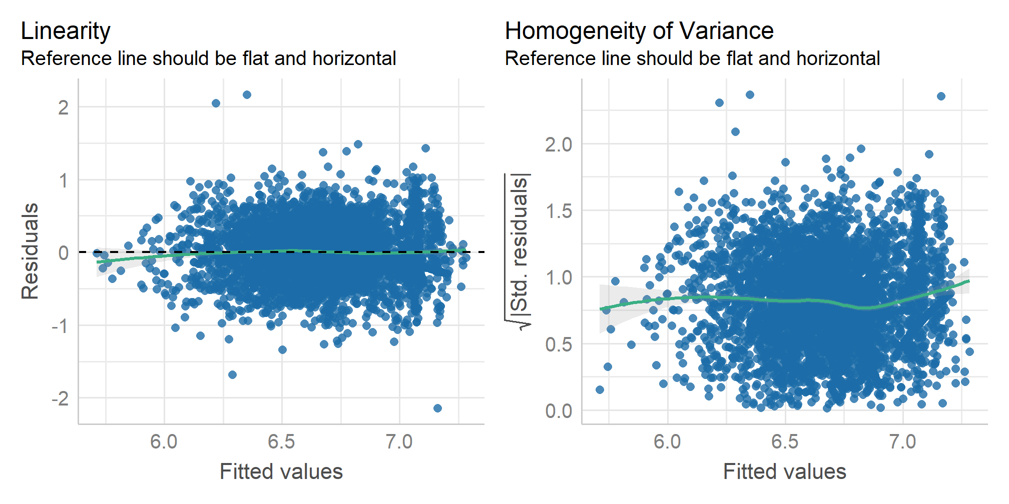
Step 1.b Assumptions (Homoscedasticity)
OK: Error variance appears to be homoscedastic (p = 0.647).Step 1.b Assumptions (Collinearity)
# Check for Multicollinearity

Low Correlation

  Term  VIF     VIF 95% CI Increased SE Tolerance Tolerance 95% CI
 union 1.11 [ 1.08,  1.15]         1.05      0.90     [0.87, 0.93]
  educ 1.13 [ 1.10,  1.18]         1.06      0.88     [0.85, 0.91]
 hours 1.03 [ 1.01,  1.09]         1.02      0.97     [0.92, 0.99]

High Correlation

       Term   VIF     VIF 95% CI Increased SE Tolerance Tolerance 95% CI
      exper 18.81 [17.73, 19.95]         4.34      0.05     [0.05, 0.06]
 I(exper^2) 18.81 [17.73, 19.95]         4.34      0.05     [0.05, 0.06]
Step 1.b Assumptions (No endogeneity)
\[ log(\text{Wage}_{it}) = \beta_0 + \beta_1 \cdot \text{Union}_{it} + \beta_2 \cdot {X_{it}} + \beta_3 \cdot \text{Ability}_{i} + \epsilon_{it} \]
\(\text{Ability}_{i}\) not observable and not measurable.
Omitting the ability may cause the OVB.
No endogeneity assumption cannot be satisfied.
We should exploit the panel data structure.
Step 2. FE: Fixed Effect (within)
Note, the new package: plm used for running panel regressions.
Declare data to be panel.
Check panel dimensions.
Balanced Panel: n = 595, T = 7, N = 4165Step 2. FE: Fixed Effect (within) (1)
Rerun the pooled regression with plm:
Model Formula: log(wage) ~ union + educ + exper + I(exper^2) + hours

Coefficients:
(Intercept)       union        educ       exper  I(exper^2)       hours
 4.70543801  0.12614668  0.08197441  0.04371549 -0.00069316  0.00770422
Fixed Effect (individual) model
Model Formula: log(wage) ~ union + educ + exper + I(exper^2) + hours

Coefficients:
      union       exper  I(exper^2)       hours
 0.03002946  0.11370518 -0.00042343  0.00079804
Step 2. FE: Fixed Effect (within) (2)
Fixed Effect (time) model
Model Formula: log(wage) ~ union + educ + exper + I(exper^2) + hours

Coefficients:
      union        educ       exper  I(exper^2)       hours
 0.12428314  0.07944664  0.03582803 -0.00058079  0.00756342
Fixed Effect (Two-ways) model
Model Formula: log(wage) ~ union + educ + exper + I(exper^2) + hours

Coefficients:
      union  I(exper^2)       hours
 0.02712246 -0.00040431  0.00064611
Step 2. F-test (1)
Which model to choose: Pooled or FE?
Compares FE models (individual, time, two-ways) vs pooled
- Pooled is always consistent vs FE
Test logic:
H0: One model is inconsistent. (no individual/time/two-way effects)
H1: Both models are equally consistent.
Run the test. Check the p-value
p-value < 0.05: FE is as good as pooled. Not using the FE model may lead to the bias.
p-value >= 0.05: Pooled is better than the FE model. Use pooled for interpretation.
Step 2. F-test (2)
- FE is preferred (pooled is biased)
- Time FE is preferred (pooled is biased)
F-testleads us to stick with the FE individual, two-ways or time regression.
Step 2. LM test: Lagrange multiplier test (2)
Which FE model to choose: individual, time or two-way?
Exist to compare FE models between each other assuming that:
- Pooled is always consistent in pooled vs individual FE
- Individual FE always consistent in individual FE vs time or two-way FE
Test logic:
- H0: One model is inconsistent.
- H1: Both models are equally consistent.
Run the test (one or another or both). Check p-value:
p-value < 0.05:
- Individual FE is as good as pooled;
- Time or Two-ways model is as good as individual FE;
p-value >= 0.05: Pooled or individual FE is better than the alternative
Step 2. LM testLagrange multiplier (2)
    Lagrange Multiplier Test - (Honda)

data:  log(wage) ~ union + educ + exper + I(exper^2) + hours
normal = 70.727, p-value < 2.2e-16
alternative hypothesis: significant effects
    Lagrange Multiplier Test - two-ways effects (Honda)

data:  log(wage) ~ union + educ + exper + I(exper^2) + hours
normal = 186.47, p-value < 2.2e-16
alternative hypothesis: significant effects
    Lagrange Multiplier Test - time effects (Honda)

data:  log(wage) ~ union + educ + exper + I(exper^2) + hours
normal = 192.98, p-value < 2.2e-16
alternative hypothesis: significant effects- Individual FE is preferred (pooled is biased)
- Individual FE and two-ways are both consistent. We can choose any of those two.
- Individual FE and time FE are both consistent. We can choose any of those two.
- All tests suggest that individual, time and two-ways fixed effect models are equally consistent.
Step 3. Random Effect model (individual)
Model Formula: log(wage) ~ union + educ + exper + I(exper^2) + hours

Coefficients:
(Intercept)       union        educ       exper  I(exper^2)       hours
 3.80500063  0.05488827  0.11346029  0.08804403 -0.00077520  0.00095463
Step 3. Hausman test
Which model to choose: Fixed effect or Random effect?
Compares Fixed Effect model with Random Effect:
- Fixed effect model is always consistent
Test logic:
H0: One model is inconsistent. Use FE!
H1: Both models are equally consistent. RE is as good as FE.
Run the test. Check the p-value.
p-value < 0.05: Use FE or RE, both are good.
p-value >= 0.05: Use FE, discard RE.
Step 4.1 Wooldridge’s test (1)
Is there serial correlation / cross-sectional dependence in the data?
Wooldridge’s test for unobserved individual effects
H0: no unobserved effects
H1: some effects exist due to cross-sectional dependence and/or serial correlation
Run the test Check the p-value.
p-value < 0.05: cross-sectional dependence and/or serial correlation are present
p-value >= 0.05: No cross-sectional dependency and/or serial correlation
Step 4.1 Wooldridge’s test (2)
    Wooldridge's test for unobserved individual effects

data:  formula
z = 13.865, p-value < 2.2e-16
alternative hypothesis: unobserved effect
    Wooldridge's test for unobserved time effects

data:  formula
z = 2.015, p-value = 0.04391
alternative hypothesis: unobserved effect- cross-sectional dependence is present
- serial correlation is present
Step 4.2 Lagrange-Multiplier tests (1)
Is there serial correlation in the data?
Locally–Robust Lagrange Multiplier Tests for serial correlation
H0: serial correlation is zero
H1: some serial correlation is present
Run the test Check the p-value.
p-value < 0.05: serial correlation need to be addressed
p-value >= 0.05: no serial correlation
Step 4.2 Lagrange-Multiplier tests (2)
Step 5. Robust inference
Serial correlation and/or cross-sectional dependence render our Standard errors useless.
Cross-sectional dependence and/or serial correlation violate the variance homogeneity assumption:
Estimates are unbiased, but inefficient.
Standard errors need to be corrected.
We need to use:
Robust Standard Errors, and/or
Clustered SE at the individual (group) level
Step 5. Robust Standard Error (1)
Model Formula: log(wage) ~ union + educ + exper + I(exper^2) + hours

Coefficients:
     union      exper I(exper^2)      hours
  0.030029   0.113705  -0.000423   0.000798
Correcting cross-sectional dependence:
Regular SE
t test of coefficients:

             Estimate Std. Error t value Pr(>|t|)
union       0.0300295  0.0148074    2.03    0.043 *
exper       0.1137052  0.0024681   46.07  < 2e-16 ***
I(exper^2) -0.0004234  0.0000546   -7.75  1.2e-14 ***
hours       0.0007980  0.0005997    1.33    0.183
---
Signif. codes:  0 '***' 0.001 '**' 0.01 '*' 0.05 '.' 0.1 ' ' 1
Robust SE
coeftest(union_fe_ind,
         vcov. = vcovHC(union_fe_ind, method = "white1",
                        type = "HC0", cluster = "group"))
t test of coefficients:

             Estimate Std. Error t value Pr(>|t|)
union       0.0300295  0.0159202    1.89    0.059 .
exper       0.1137052  0.0025948   43.82  < 2e-16 ***
I(exper^2) -0.0004234  0.0000539   -7.86  5.1e-15 ***
hours       0.0007980  0.0007524    1.06    0.289
---
Signif. codes:  0 '***' 0.001 '**' 0.01 '*' 0.05 '.' 0.1 ' ' 1
Step 5. Robust Standard Error (2)
We produce new Variance-covariance matrix:
                   union         exper      I(exper^2)           hours
union       0.0002534526 -0.0000028527  0.000000054371 -0.000000443094
exper      -0.0000028527  0.0000067329 -0.000000126361  0.000000043707
I(exper^2)  0.0000000544 -0.0000001264  0.000000002902  0.000000000683
hours      -0.0000004431  0.0000000437  0.000000000683  0.000000566054
attr(,"cluster")
[1] "group"methodsfor cross–sectional dependence “white1” and “white2” and for cross–sectional dependence and autocorrelation “arellano”;typefor sample size correction: “HC0”, “sss”, “HC1”, “HC2”, “HC3”, “HC4” (“HC3” is recommended);clusterenabled by default (“group” or “time”);
Step 6. Reporting results (1)
pooled_robust <-
  coeftest(union_pooled,
           vcov. = vcovHC(union_pooled, method = "arellano",
                          type = "HC3", cluster = "group"))

pooled_cs_robust <-
  coeftest(union_fe_ind,
           vcov. = vcovHC(union_fe_ind, method = "white1",
                          type = "HC0", cluster = "group"))

pooled_csac_robust <-
  coeftest(union_fe_ind,
           vcov. = vcovHC(union_fe_ind, method = "arellano",
type = "HC3", cluster = "group"))modelsummary(
list(
`Pooled (no SE correction)` = coeftest(union_pooled),
`Pooled (c/s dep. and aut.)` = pooled_robust,
`Ind. FE (no SE correction)` = coeftest(union_fe_ind),
`Ind. FE (c/s dep.)` = pooled_cs_robust,
`Ind. FE (c/s dep. and aut.)` = pooled_csac_robust
),
fmt = 4, statistic = NULL,
estimate = "{estimate}{stars} ({std.error})")Step 6. Reporting results (1)
| Pooled (no SE correction) | Pooled (c/s dep. and aut.) | Ind. FE (no SE correction) | Ind. FE (c/s dep.) | Ind. FE (c/s dep. and aut.) | |
|---|---|---|---|---|---|
| (Intercept) | 4.7054*** (0.0699) | 4.7054*** (0.1383) | |||
| union | 0.1261*** (0.0131) | 0.1261*** (0.0255) | 0.0300* (0.0148) | 0.0300+ (0.0159) | 0.0300 (0.0256) |
| educ | 0.0820*** (0.0023) | 0.0820*** (0.0052) | |||
| exper | 0.0437*** (0.0024) | 0.0437*** (0.0053) | 0.1137*** (0.0025) | 0.1137*** (0.0026) | 0.1137*** (0.0040) |
| I(exper^2) | −0.0007*** (0.0001) | −0.0007*** (0.0001) | −0.0004*** (0.0001) | −0.0004*** (0.0001) | −0.0004*** (0.0001) |
| hours | 0.0077*** (0.0012) | 0.0077*** (0.0019) | 0.0008 (0.0006) | 0.0008 (0.0008) | 0.0008 (0.0009) |
| Num.Obs. | 4165 | 4165 | 4165 | 4165 | 4165 |
| AIC | 3911.1 | 3911.1 | −4502.1 | −4502.1 | −4502.1 |
| BIC | 3955.5 | 3955.5 | −4470.5 | −4470.5 | −4470.5 |
| Log.Lik. | -1948.564 | -1948.564 | 2256.066 | 2256.066 | 2256.066 |
Step 6. Reporting GOF (1)
# Comparison of Model Performance Indices

Name   | Model |   AIC (weights) |  AICc (weights) |   BIC (weights) |    R2 | R2 (adj.) |  RMSE | Sigma
--------------------------------------------------------------------------------------------------------
Pooled |   plm | 59525.1 (<.001) | 59525.1 (<.001) | 59569.4 (<.001) | 0.299 |     0.298 | 0.386 | 0.387
FE     |   plm | 51111.8 (>.999) | 51111.8 (>.999) | 51143.5 (>.999) | 0.657 |     0.600 | 0.141 | 0.141
Takeaways
Takeaways for the exam
Simpson’s paradox. What are the causes of it and solutions.
Data types (cross-section, repeated cross-section, balanced panel, unbalanced panel)
Panel Regression
- Pooled;
- Least Squared Dummy Variable model;
- Fixed effect (within transformation);
- Why FE is so important?
- What is the key difference between FE and RE?
- When FE and when RE are appropriate?
Panel Regression tests
F-test,LM-test,Hausman testRobust and Clustered SE:
- Why these are important and when do we need to use one?
Homework
Reproduce code from the slides
Perform practical exercises.