Interaction terms in MLR and Difference in Difference (DID)

Author

Affiliation

Eduard Bukin

Institute of Agricultural Policy and Market Research. Faculty 09. Justus Liebig University Giessen.

MLR with an interaction term

Interaction term

\[ y = \beta_0 + \beta_1 x_1 + \beta_2 x_2 + \beta_3 (x_1 \cdot x_2) + \beta_4 x_4 + \epsilon \]

Interpretation is only possible through marginal effects:

Marginal effect is a partial derivative of the regression equation with respect to a regressor of interest evaluated at certain value of the interaction term.

\(\frac{\partial y}{\partial x_1} = \beta_1 + \beta_3 x_2\)

\(\frac{\partial y}{\partial x_2} = \beta_2 + \beta_3 x_1\)

Marginal Effect (the slope) of \(x_1\) depends on \(x_2\) and vice versa.

Reporting results with marginal effects

Report coefficients \(\beta_1\), \(\beta_2\), \(\beta_3\) as is.
Report marginal effects at mean values of the interaction term(s):
- \(\text{ME}(\bar x_1) = \beta_1 + \beta_3 \bar x_2\)
- \(\text{ME}(\bar x_2) = \beta_2 + \beta_3 \bar x_1\)
To compute standard errors for the marginal effects, we use delta method.

Learn more: (Angrist & Pischke, 2009, also Chapter 3)

Recall the hedonic land prices model:

\[ \text{acrePrice} = \beta_0 + \beta_1 \text{crpPct} + \beta_2 \text{acres} + \beta_3 \text{improvements} \\ + \beta_4 \text{year} + \beta_5 \text{region} + e \]

acrePrice - sale price in dollars per acre;
crpPct - the percentage of all farm acres enrolled in CRP;
acres - size of the farm in acres;
improvements - share of infrastructure’s value in the land price;
development - dummy variable aliased with improvements. Is 1 when improvements > 25% and is 0 otherwise.
region - region in the state Minnesota;
year - year of the land sales translation;

Loading data

Warning: package 'modelsummary' was built under R version 4.2.3

Warning: package 'marginaleffects' was built under R version 4.2.3

Warning: package 'GGally' was built under R version 4.2.3

Registered S3 method overwritten by 'GGally':
  method from   
  +.gg   ggplot2

Warning in mask$eval_all_mutate(quo): NAs introduced by coercion

Warning in mask$eval_all_mutate(quo): NAs introduced by coercion

Warning in mask$eval_all_mutate(quo): NAs introduced by coercion

Show the code

library(tidyverse)
library(readxl)
library(modelsummary)
library(ggeffects)
library(marginaleffects)
library(GGally)
options(modelsummary_get = "broom")
## 1. Load the data
dta <- read_excel("land-prices.xlsx") %>%
  mutate(improvements  = as.numeric(improvements),
         development = as.factor(as.integer(improvements > 25)),
         productivity  = as.numeric(productivity),
         tillable  = as.numeric(tillable),
         year = as.factor(year)) %>% 
  select(acrePrice, crpPct, acres, improvements, development, region, year)

glimpse(dta)

Descriptive statistics

Show the code

datasummary(
    acrePrice + crpPct + acres + improvements + as.integer(development) ~ 
      (mean + sd + min + median + max) * 
      Arguments(na.rm = TRUE),
    data = dta, 
    output = "html"
  )

	mean	sd	min	median	max
acrePrice	2787.33	1914.04	108.00	2442.00	15000.00
crpPct	4.16	17.17	0.00	0.00	100.00
acres	112.69	128.46	1.00	80.00	6970.00
improvements	4.49	12.94	0.00	0.00	100.00
as.integer(development)	1.08	0.26	1.00	1.00	2.00

Descriptive Plots

Show the code

dta %>%
  select(acrePrice, crpPct, acres, improvements, development) %>%
  ggpairs(aes(colour = development, alpha = 0.2))

Warning in ggally_statistic(data = data, mapping = mapping, na.rm = na.rm, :
Removed 50 rows containing missing values

Warning in ggally_statistic(data = data, mapping = mapping, na.rm = na.rm, :
Removed 50 rows containing missing values

Warning in ggally_statistic(data = data, mapping = mapping, na.rm = na.rm, :
Removed 50 rows containing missing values

Warning in ggally_statistic(data = data, mapping = mapping, na.rm = na.rm, :
Removed 50 rows containing missing values

Warning in ggally_statistic(data = data, mapping = mapping, na.rm = na.rm, :
Removed 50 rows containing missing values

Warning in ggally_statistic(data = data, mapping = mapping, na.rm = na.rm, :
Removed 50 rows containing missing values

Warning: Removed 50 rows containing missing values (`geom_point()`).
Removed 50 rows containing missing values (`geom_point()`).
Removed 50 rows containing missing values (`geom_point()`).

Warning: Removed 50 rows containing non-finite values (`stat_density()`).

Warning: Removed 50 rows containing non-finite values (`stat_boxplot()`).

`stat_bin()` using `bins = 30`. Pick better value with `binwidth`.
`stat_bin()` using `bins = 30`. Pick better value with `binwidth`.
`stat_bin()` using `bins = 30`. Pick better value with `binwidth`.
`stat_bin()` using `bins = 30`. Pick better value with `binwidth`.

Warning: Removed 50 rows containing non-finite values (`stat_bin()`).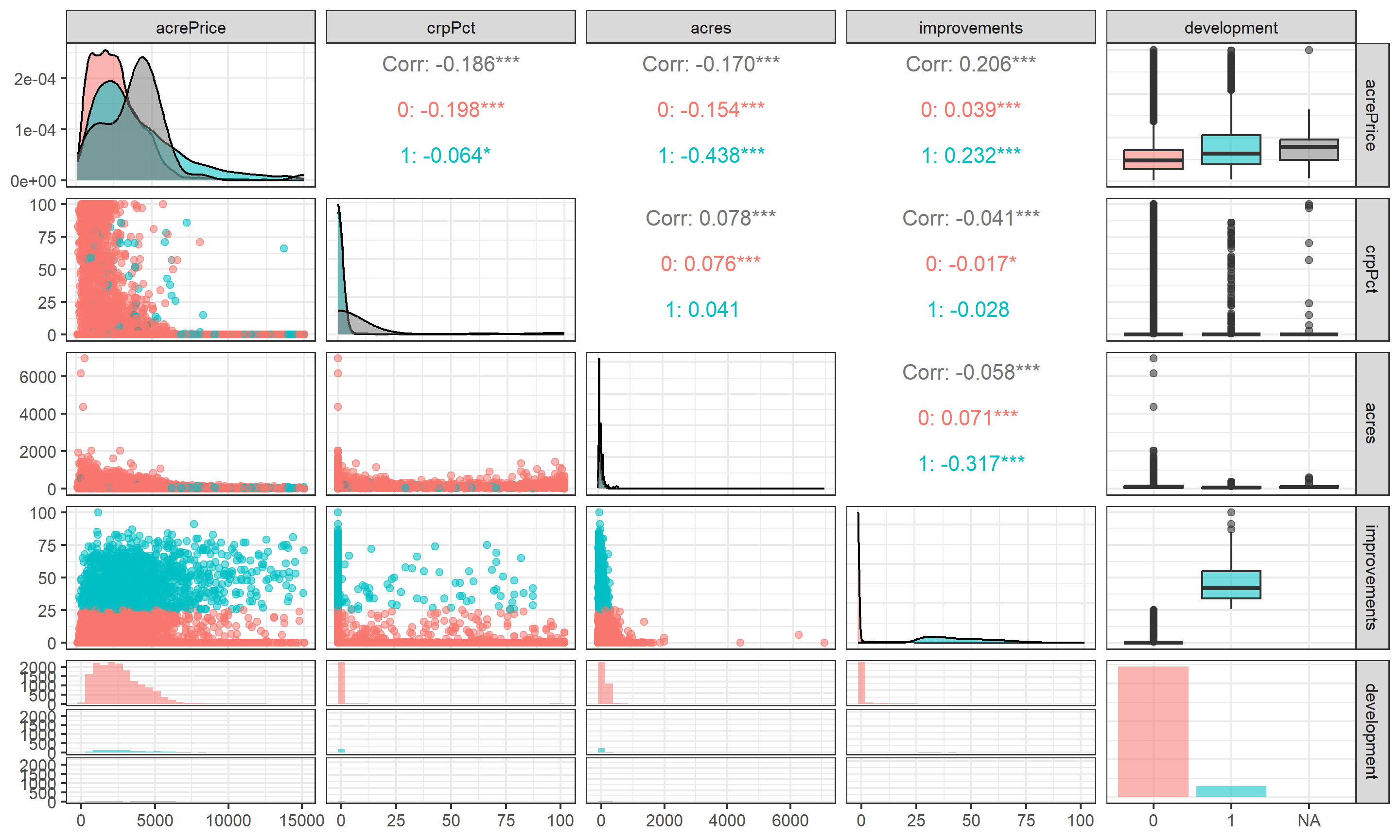

Example 1. Basic regressions

Show the code

fit1 <- 
  lm(acrePrice  ~ acres + development + crpPct + region + factor(year),
     data = dta)

summ <-
  function(x, coef_omit = "reg|year", output = "html", notes = NULL, ...) {
    modelsummary(
      x,
      estimate = "{estimate}{stars} ({std.error})",
      statistic = NULL,
      output = output,
      gof_omit =  c("AIC|BIC|Log|F|RMS"),
      coef_omit = coef_omit,
      notes = notes,
      ...
    )
  }

cust_summ <- function(x, coef_omit = "reg|year", output = "markdown", ...) {
  x <- set_names(x, str_c("Model ", seq_along(x)))
  all_eq <- x %>% imap_chr(. , ~ {str_c(.y, ": ", as.character(.x$call)[[2]])}) %>% 
    str_c(collapse = "</br>")
  summ(x, coef_omit = coef_omit, output = output, notes = all_eq, ...)
}

Interpret the baseline results

Show the code

cust_summ(list(fit1))

	Model 1
(Intercept)	2019.877*** (65.416)
acres	-0.857*** (0.086)
development1	1555.287*** (41.467)
crpPct	-8.892*** (0.645)
:————-	———————:
Num.Obs.	18650
R2	0.413
R2 Adj.	0.412

Note: ^^ Model 1: acrePrice ~ acres + development + crpPct + region + factor(year)

Fitted vs area and development

Show the code

library(ggeffects)
ggpredict(fit1, terms = "acres") %>%
  plot() + 
  ylab("Predicted price per acre (acrePrice), USD")+ 
  xlab("Parcel size (acres), acres")

Show the code

ggpredict(fit1, terms = "development") %>%
  plot() + 
  ylab("Predicted price per acre (acrePrice), USD")+ 
  xlab("Development, 0 = no 1 = yes")

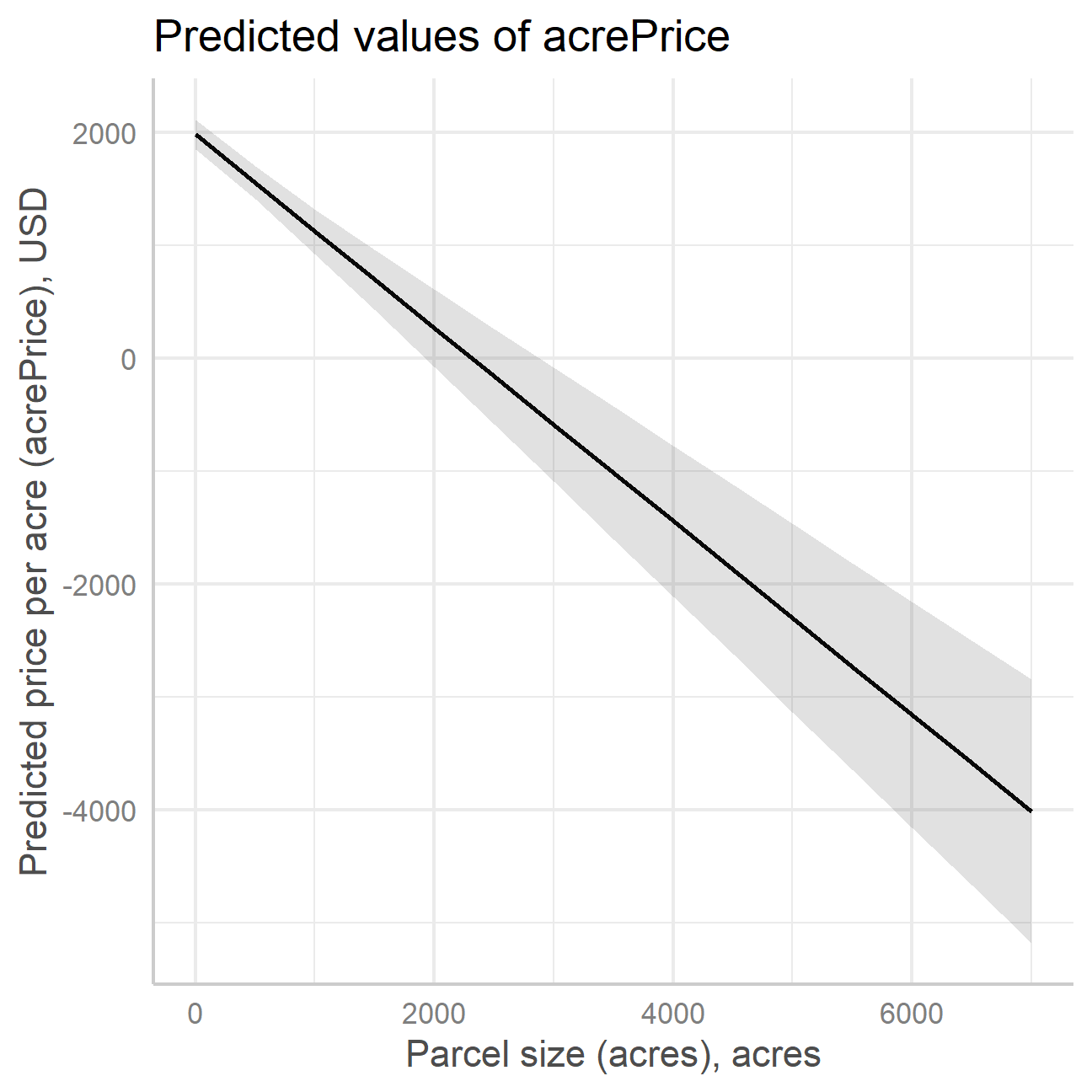
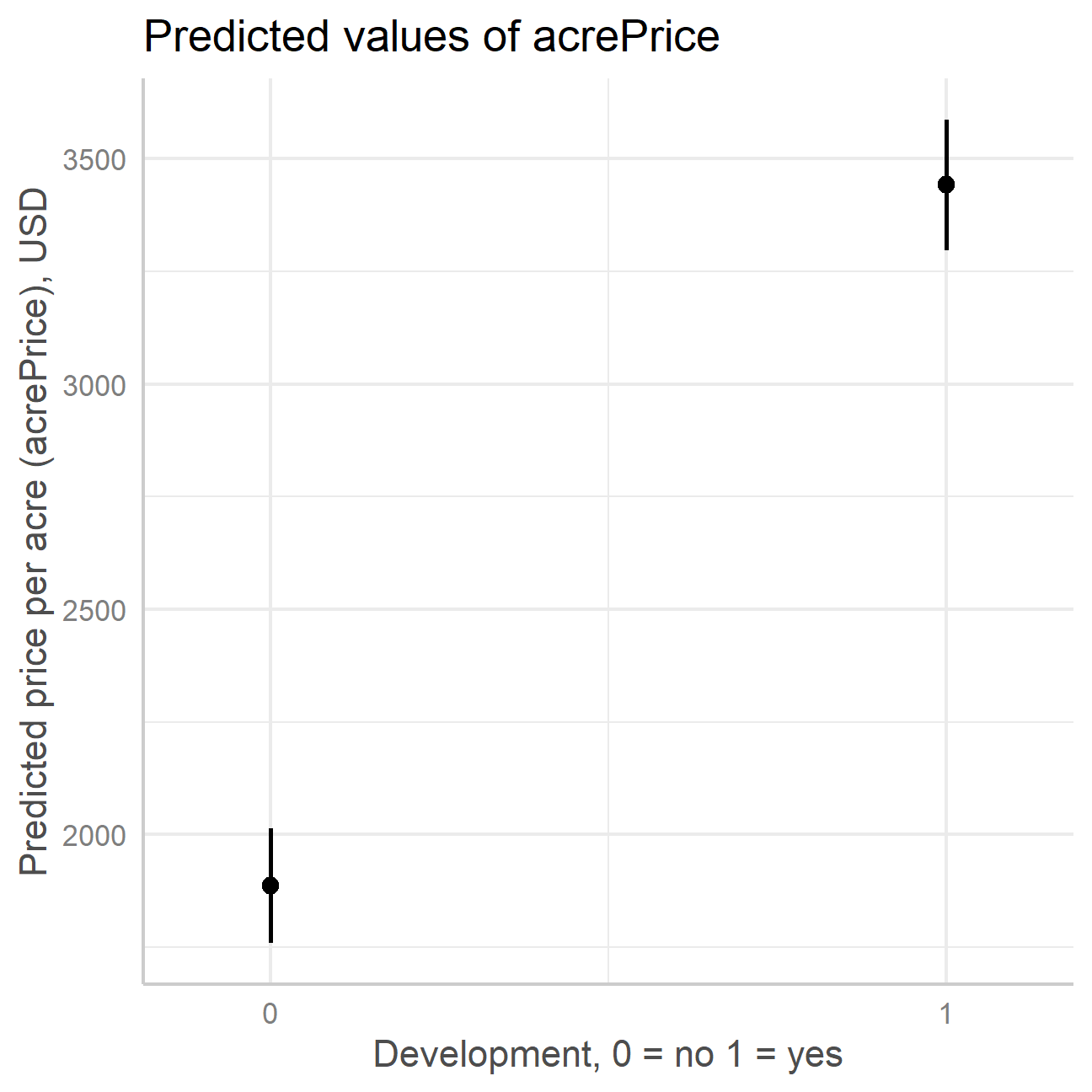
Fitted vs area and development (2)

Show the code

ggpredict(fit1, terms = c("acres", "development")) %>%
  plot() + 
  ylab("Predicted price per acre (acrePrice), USD") + 
  xlab("Parcel size (acres), acres")

Without an interaction term, dummy variables simply cause shifts in the outcome variable.

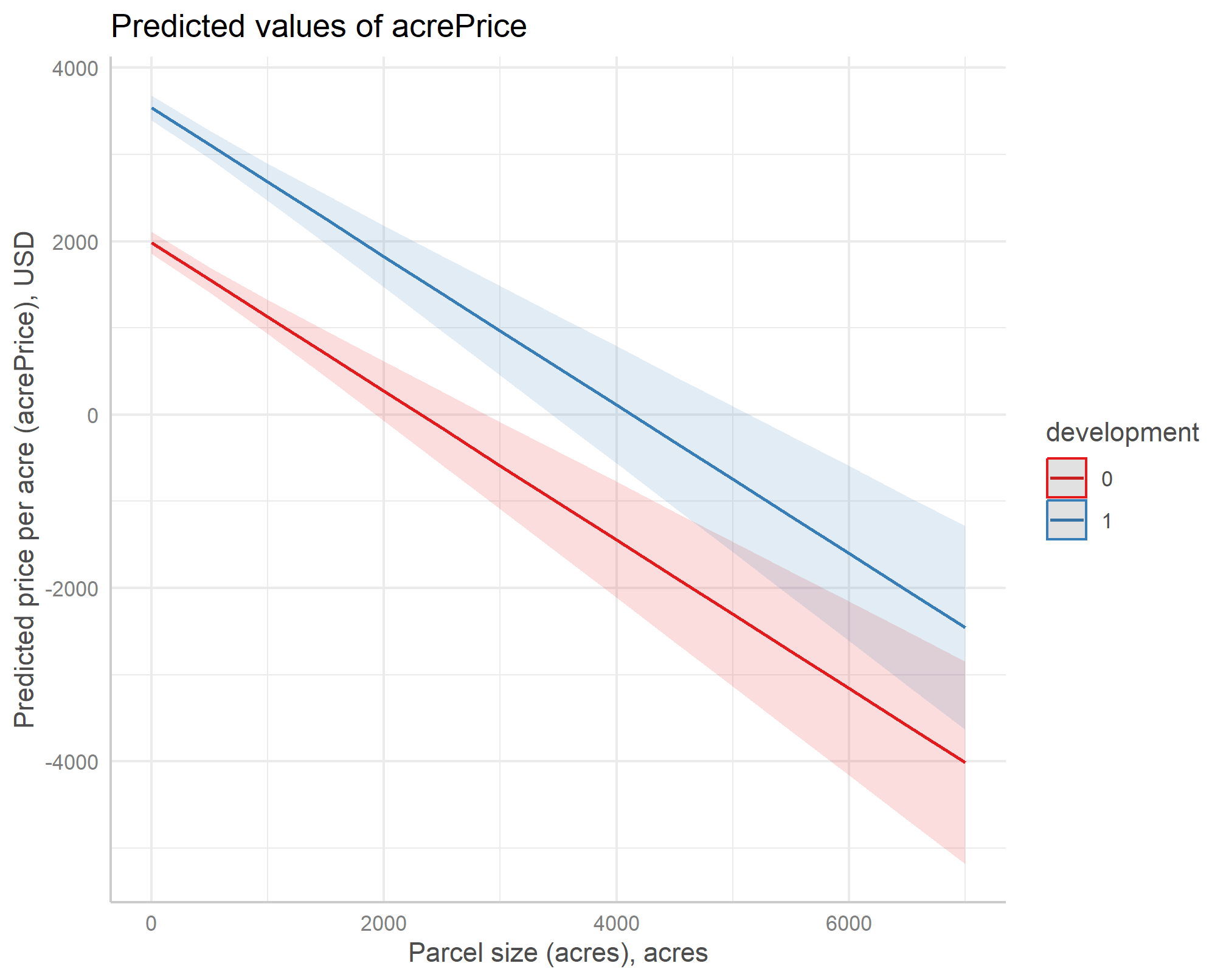
Example 2. Interaction term with a binary variable

Show the code

fit2 <- 
  lm(acrePrice  ~ acres * development + crpPct + region + factor(year),
     data = dta)
cust_summ(list(fit1, fit2))

	Model 1	Model 2
(Intercept)	2019.877*** (65.416)	1997.055*** (64.413)
acres	-0.857*** (0.086)	-0.652*** (0.085)
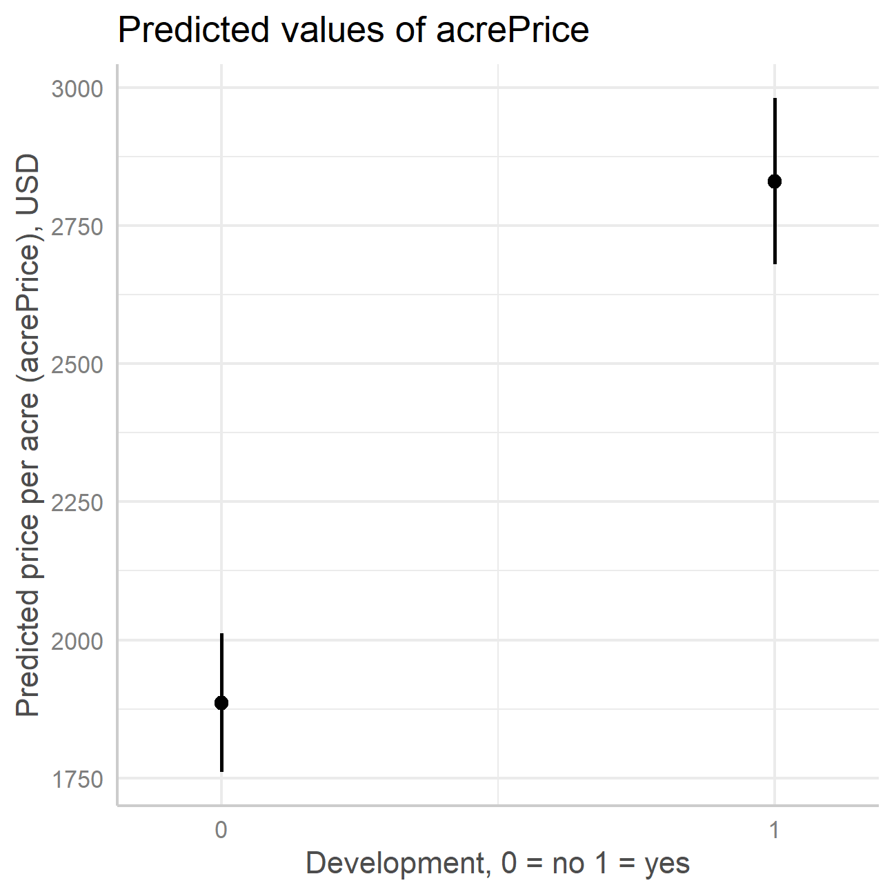
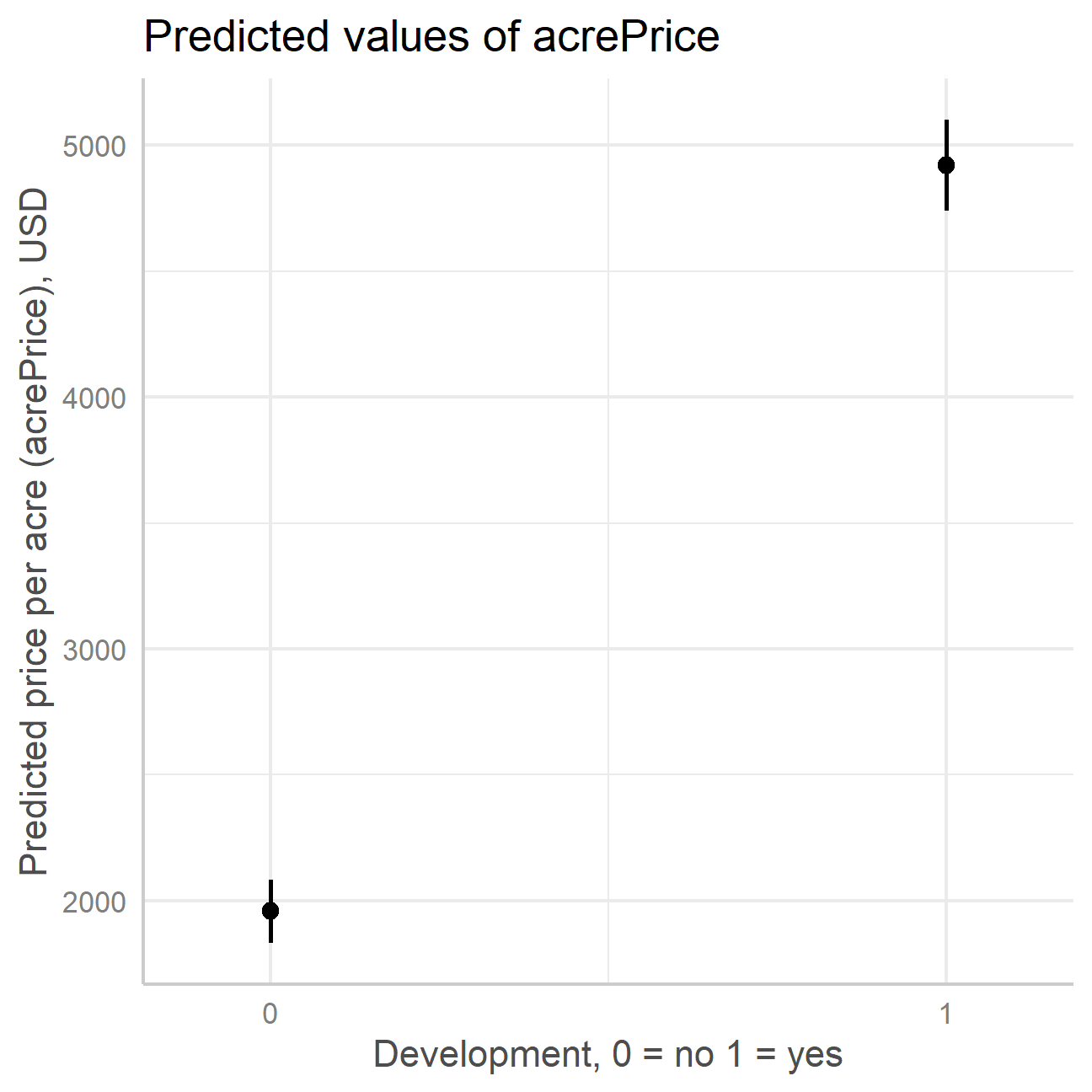
development1	1555.287*** (41.467)	2978.491*** (71.424)
crpPct	-8.892*** (0.645)	-9.073*** (0.635)
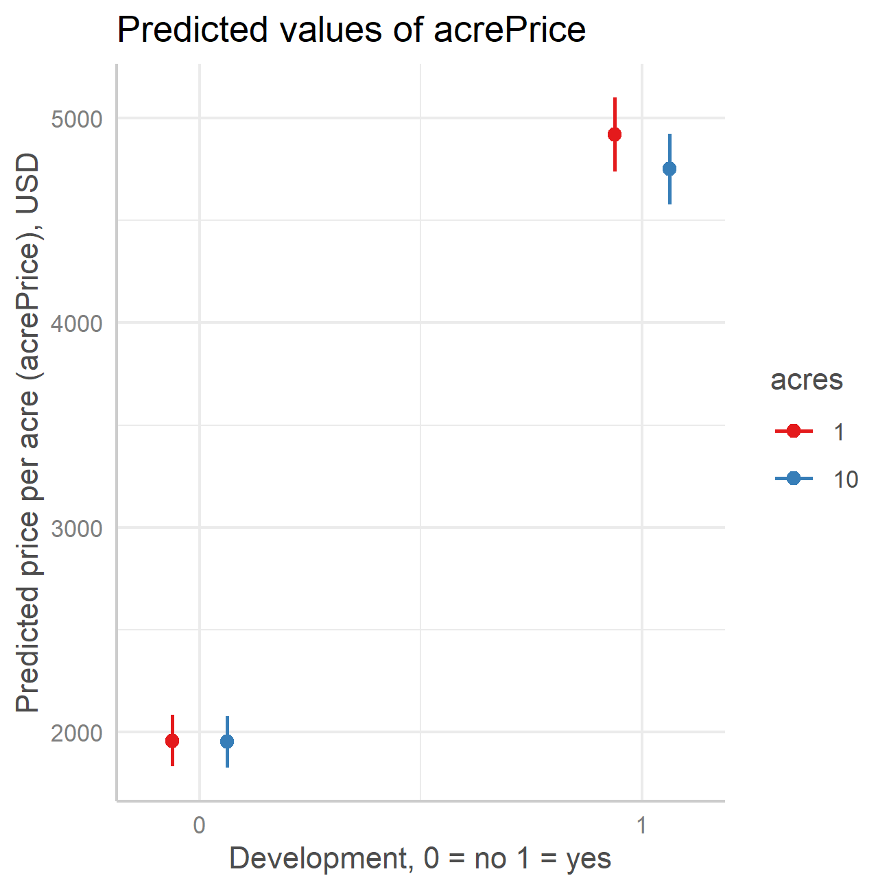
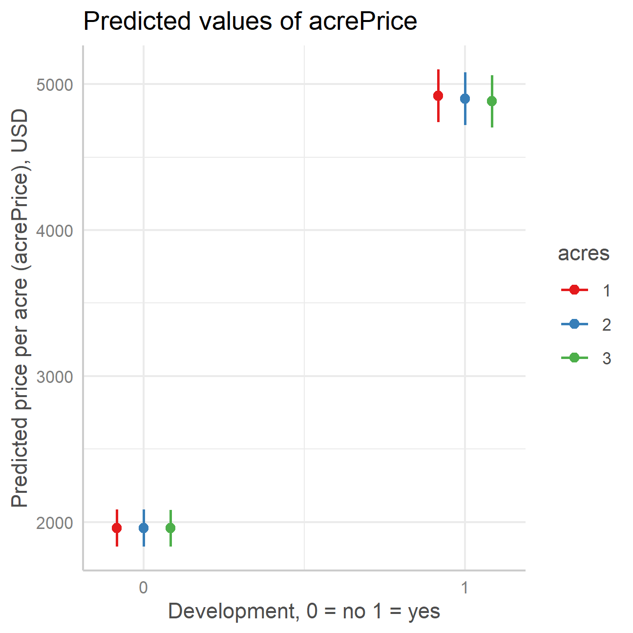
acres × development1		-18.053*** (0.743)
:———————	———————:	———————:
Num.Obs.	18650	18650
R2	0.413	0.431
R2 Adj.	0.412	0.430

Note: ^^ Model 1: acrePrice ~ acres + development + crpPct + region + factor(year)
Model 2: acrePrice ~ acres * development + crpPct + region + factor(year)

Fitted vs development with an interaction term

Show the code

ggpredict(fit2, terms = c("development")) %>%
  plot() + 
  ylab("Predicted price per acre (acrePrice), USD") + 
  xlab("Development, 0 = no 1 = yes")

Show the code

ggpredict(fit2, terms = c("development", "acres [0, 10, 50, 100, 200, 250, 500]")) %>%
  plot() + 
  ylab("Predicted price per acre (acrePrice), USD") + 
  xlab("Development, 0 = no 1 = yes")

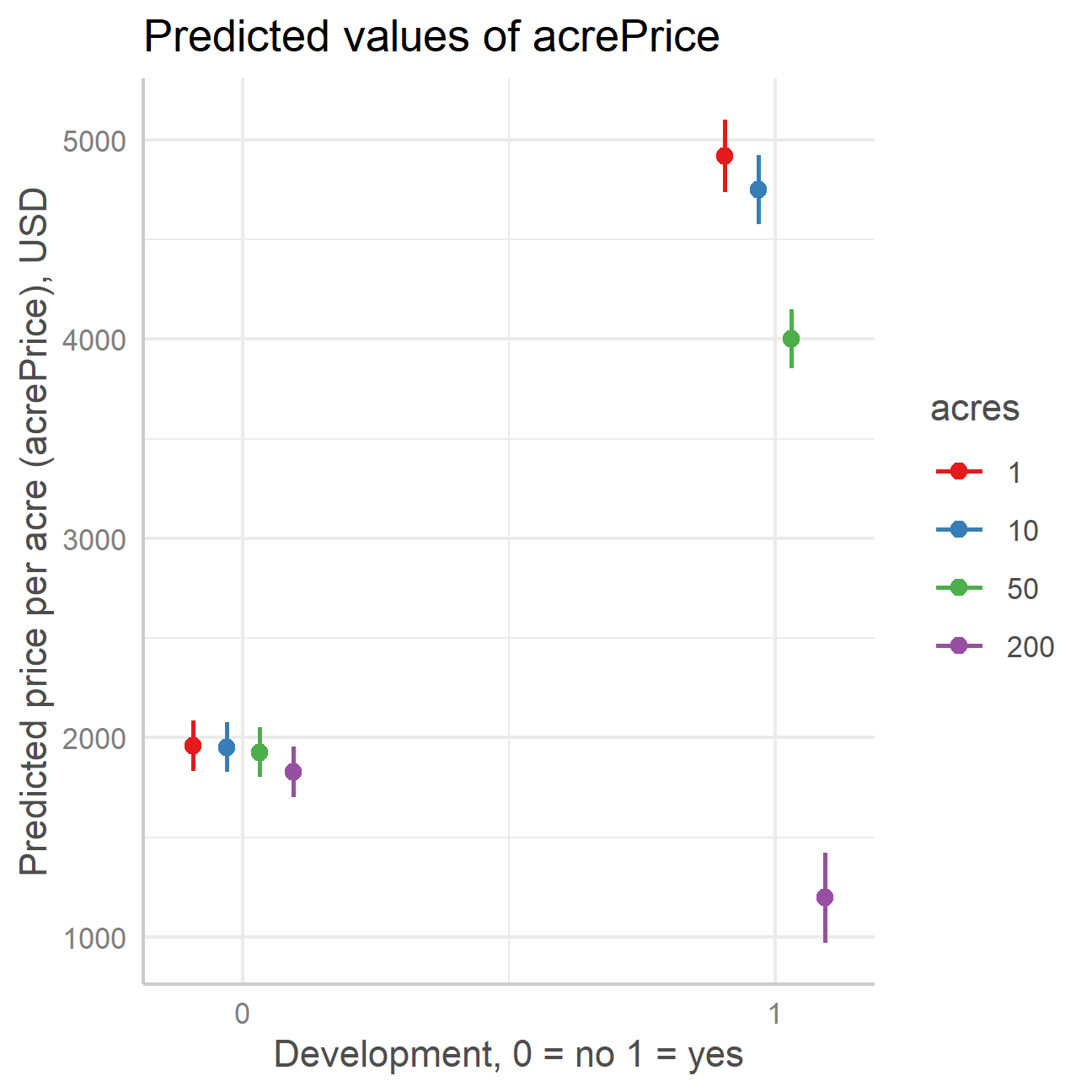
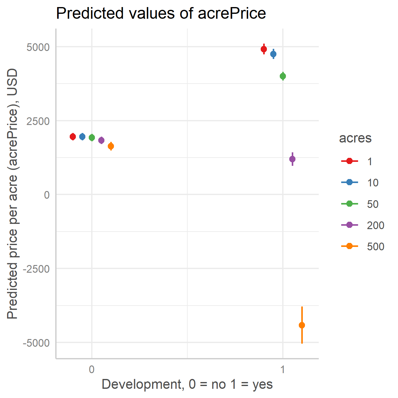
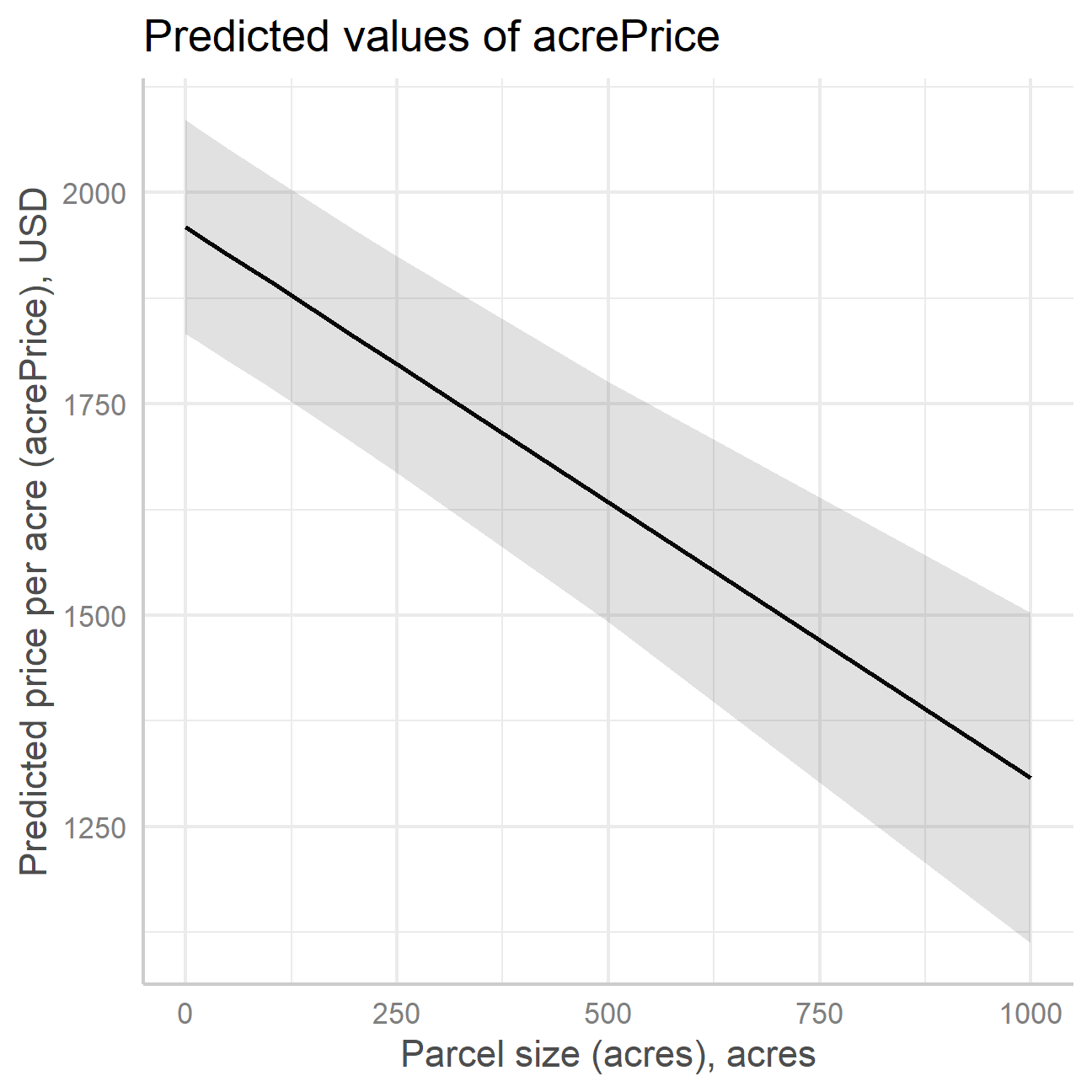
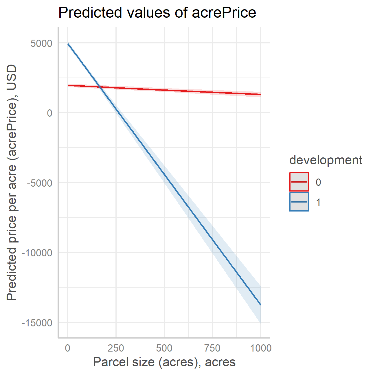
Fitted vs area with an interaction term

Show the code

ggpredict(fit2, terms = c("acres [0, 10, 50, 100, 200, 250, 500, 1000]")) %>%
  plot() + 
  ylab("Predicted price per acre (acrePrice), USD") + 
  xlab("Parcel size (acres), acres")

Show the code

ggpredict(fit2, terms = c("acres [0, 10, 50, 100, 200, 250, 500, 1000]", "development")) %>%
  plot() + 
  ylab("Predicted price per acre (acrePrice), USD") + 
  xlab("Parcel size (acres), acres")

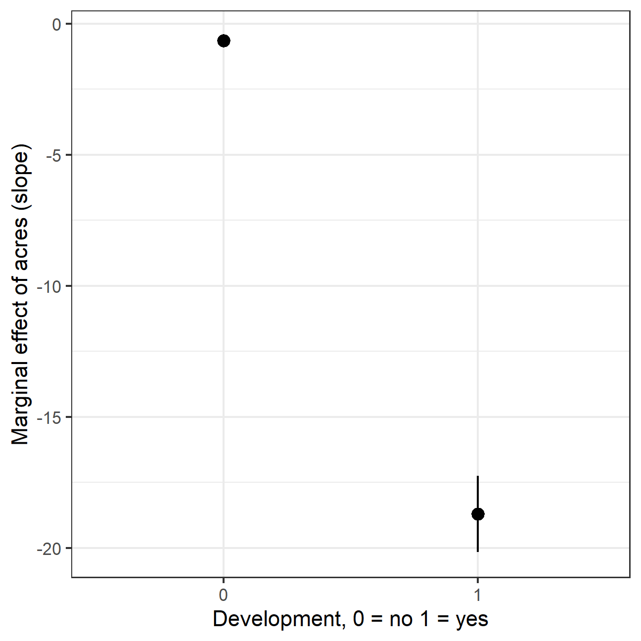
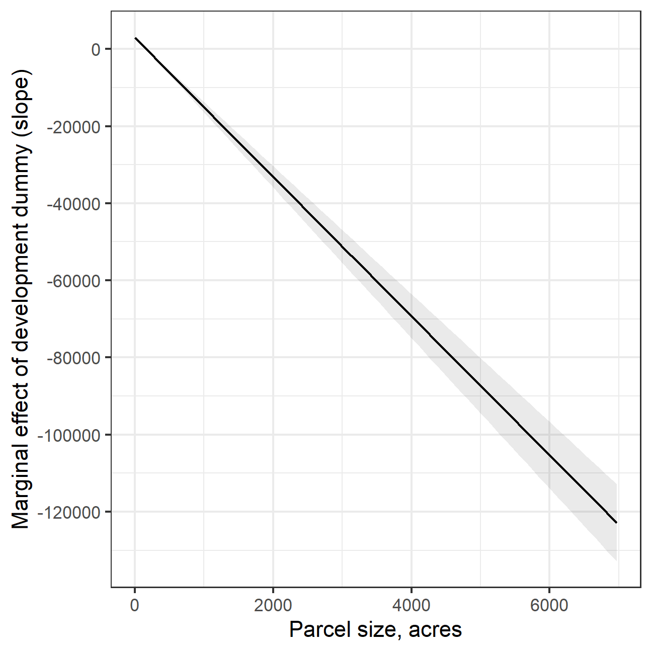
Marginal Effect `acres` and `development` at means

Show the code

library(marginaleffects)
modelsummary(fit2)
modelsummary(marginaleffects(fit2))

Show the code

summ(
  list(`Coef. as is` = fit2,
       `M.E. at means` = marginaleffects(fit2)),
  output = "html",
  coef_map = c(
    "acres" = "acres",
    "crpPct" = "crpPct",
    "development" = "development1",
    "development1" = "development1",
    "acres:development1" = "acres * development1"
  )
)

	Coef. as is	M.E. at means
acres	−0.652*** (0.085)	−2.017*** (0.097)
crpPct	−9.073*** (0.635)	−9.073*** (0.635)
development1	2978.491*** (71.424)	944.727*** (47.947)
acres * development1	−18.053*** (0.743)
Num.Obs.	18650	18650
R2	0.431	0.431
R2 Adj.	0.430	0.430

Marginal Effect `acres` and `development` (visually)

Show the code

plot_slopes(fit2, variables = "acres", condition = "development") + 
  ylab("Marginal effect of acres (slope)") + xlab("Development, 0 = no 1 = yes")

Show the code

plot_slopes(fit2, variables = "development", condition = "acres") + 
  ylab("Marginal effect of development dummy (slope)") + xlab("Parcel size, acres") + 
  scale_y_continuous(n.breaks = 10)

Example 3. Interaction with a continuous variable

Show the code

fit3 <- 
  lm(acrePrice  ~ acres * improvements + crpPct + region + factor(year),
     data = dta)
cust_summ(list(fit1, fit2, fit3), output = "markdown")

	Model 1	Model 2	Model 3
(Intercept)	2019.877*** (65.416)	1997.055*** (64.413)	1923.131*** (64.085)
acres	-0.857*** (0.086)	-0.652*** (0.085)	-0.276** (0.089)
development1	1555.287*** (41.467)	2978.491*** (71.424)
crpPct	-8.892*** (0.645)	-9.073*** (0.635)	-8.980*** (0.631)
acres × development1		-18.053*** (0.743)
improvements			56.695*** (1.307)
acres × improvements			-0.277*** (0.014)
:———————	———————:	———————:	———————:
Num.Obs.	18650	18650	18650
R2	0.413	0.431	0.438
R2 Adj.	0.412	0.430	0.438

Note: ^^ Model 1: acrePrice ~ acres + development + crpPct + region + factor(year)
Model 2: acrePrice ~ acres * development + crpPct + region + factor(year)
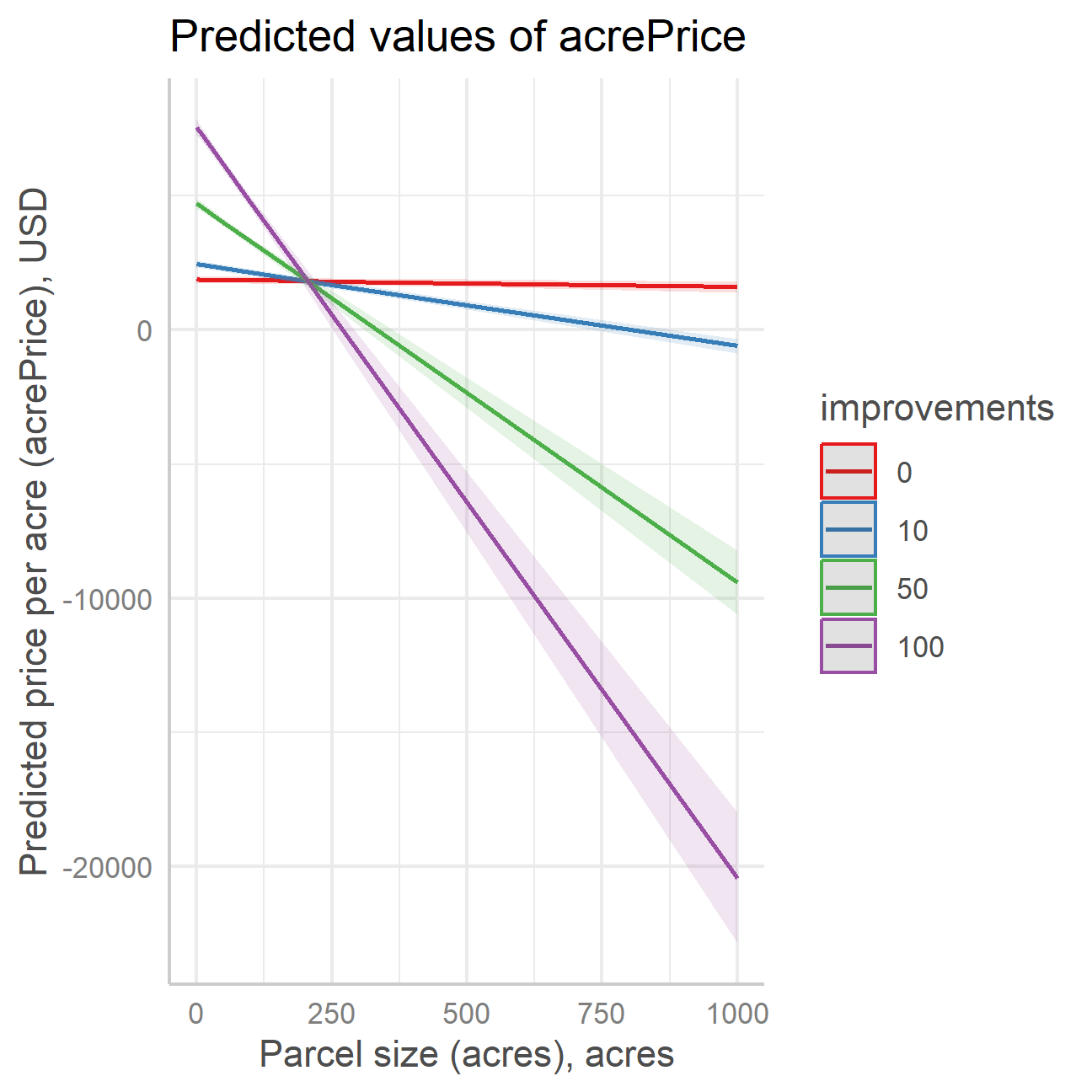
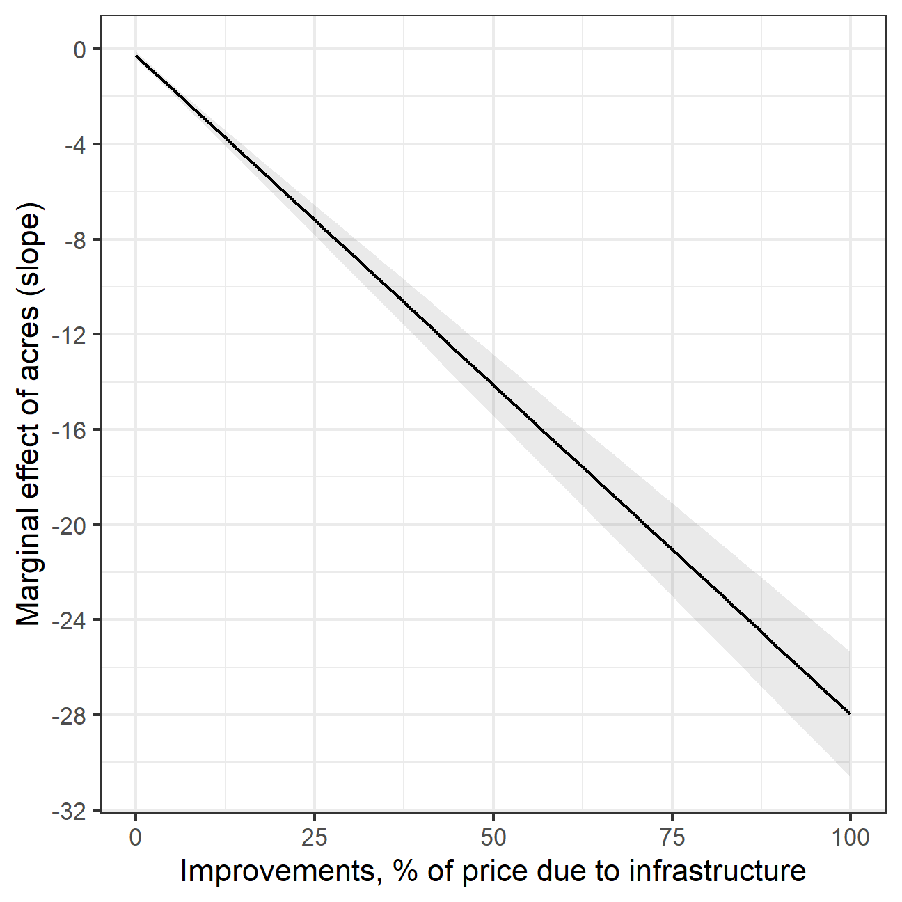
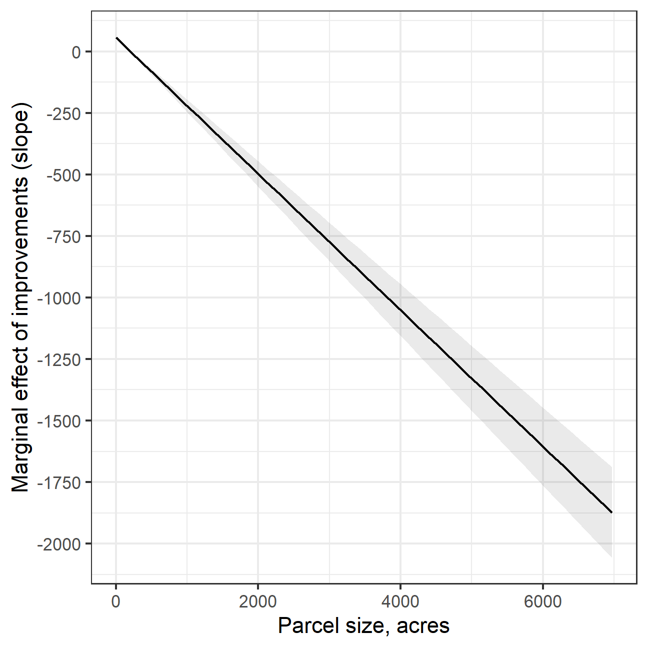
Model 3: acrePrice ~ acres * improvements + crpPct + region + factor(year)

Fitted vs `area` * `improvements`

Show the code

ggpredict(fit3, terms = c("acres [0, 10, 50, 100, 200, 250, 500, 1000]", "improvements [0, 10, 50, 100]")) %>%
  plot() + 
  ylab("Predicted price per acre (acrePrice), USD") + 
  xlab("Parcel size (acres), acres")

Show the code

ggpredict(fit3, terms = c("improvements", "acres [1, 50, 100, 200, 500]")) %>%
  plot() + 
  ylab("Predicted price per acre (acrePrice), USD") + 
  xlab("Improvements, % of price due to infrastructure")

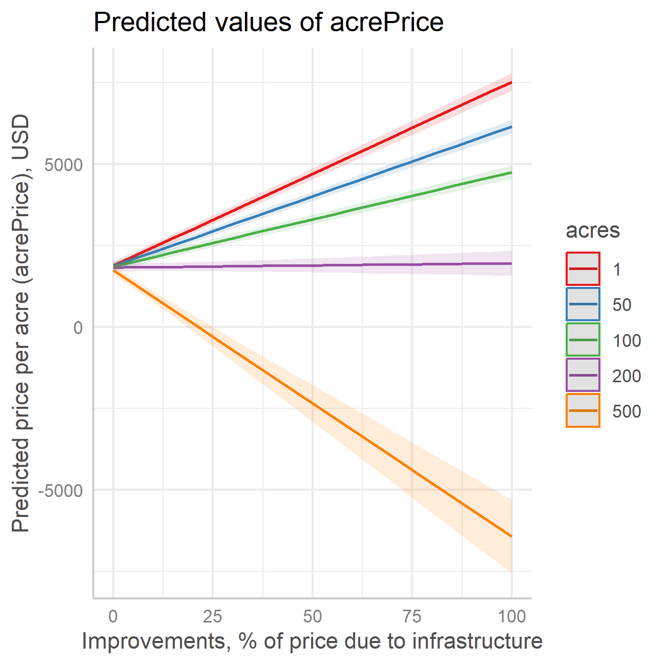
Marginal Effect `acres` * `improvements` (visually)

Show the code

plot_slopes(fit3, variables = "acres", condition = "improvements") + 
  ylab("Marginal effect of acres (slope)")  + 
  xlab("Improvements, % of price due to infrastructure")  + 
  scale_y_continuous(n.breaks = 10)

Show the code

plot_slopes(fit3, variables = "improvements", condition = "acres") + 
  ylab("Marginal effect of improvements (slope)") + xlab("Parcel size, acres") + 
  scale_y_continuous(n.breaks = 10)

Reporting all regressions results

Show the code

modelsummary(
  list(
    `Model 1 (no interaction)` = fit1,
    `Model 2 (Area*Development)` = marginaleffects(fit2, vcov = ~ region),
    `Model 3 (Area*Improvements)` = slopes(fit3, vcov = ~ region)
    ),
  vcov = list(~ region, NULL, NULL),
  estimate = "{estimate}{stars} ({std.error})",
  statistic = NULL,
  gof_omit =  c("AIC|BIC|Log|F|RMS|Std"),
  output = "html",
  coef_map = c(
    "acres" = "Area, acres (*)",
    "crpPct" = "crpPct",
    "development" = "Development status, dummy (*)",
    "improvements" = "Share infrastructure in land price, % (*)"
  ), 
  notes = "(*) marginal effects of the coefficients are reported at means of the corresponding interaction terms. Robust standard errors clustered at region are reported in brackets. For marginal effects, standard errors are estimated using delta method."
)

	Model 1 (no interaction)	Model 2 (Area*Development)	Model 3 (Area*Improvements)
Area, acres (*)	−0.857* (0.350)	−2.017*** (0.097)	−1.520*** (0.089)
crpPct	−8.892*** (1.998)	−9.073*** (0.635)	−8.980*** (0.631)
Development status, dummy (*)		944.727*** (47.947)
Share infrastructure in land price, % (*)			25.490*** (0.984)
Num.Obs.	18650	18650	18650
R2	0.413	0.431	0.438
R2 Adj.	0.412	0.430	0.438
(*) marginal effects of the coefficients are reported at means of the corresponding interaction terms. Robust standard errors clustered at region are reported in brackets. For marginal effects, standard errors are estimated using delta method.

Takeaway and homework

Marginal effects.
Difference between fitted values and marginal effects.
Homework:
- Reproduce code from the slides.
- Follow pre-recorded materials with extra calculations.

References

Angrist, J. D., & Pischke, J.-S. (2009). Mostly harmless econometrics. Princeton University Press. http://doi.org/10.1515/9781400829828

MLR with an interaction term

Interaction term

Reporting results with marginal effects

Recall the hedonic land prices model:

Loading data

Descriptive statistics

Descriptive Plots

Example 1. Basic regressions

Interpret the baseline results

Fitted vs area and development

Fitted vs area and development (2)

Example 2. Interaction term with a binary variable

Fitted vs development with an interaction term

Fitted vs area with an interaction term

Marginal Effect acres and development at means

Marginal Effect acres and development (visually)

Example 3. Interaction with a continuous variable

Fitted vs area * improvements

Marginal Effect acres * improvements (visually)

Reporting all regressions results

Takeaway and homework

Takeaway and homework

References

References

Marginal Effect `acres` and `development` at means

Marginal Effect `acres` and `development` (visually)

Fitted vs `area` * `improvements`

Marginal Effect `acres` * `improvements` (visually)