Multiple Linear Regression: practical aspects

Eduard Bukin

Relevance of a theory in econometric models

The Basic Theory of Production (Sadoulet & de Janvry, 1995, Chapter 3)

Farm’s production function

\[ h(q,x,z) = 0, \]

where:

  • \(q\) - output quantities (agricultural produce)

  • \(x\) - variable input quantities (fertilizers, labor, seed, water, …)

  • \(z\) - fixed factors (private: land, equipment; public: infrastructure, extension; exogenous features …)

Farm’s optimization problem

Prices of inputs \(w^{'}\) and outputs \(p^{'}\) affect farmers decisions of:

  • what and how much to produce \(q\), and

  • what and how much to use as the input \(x\).

Farm’s objective function is to maximize own profit:

\[ \max_{x,q} \;\;\; p^{'}q-w^{'}x, \\ \text{s.t.} \;\; h(q,x,z) = 0 \]

Solution to the producer’s optimization problem

\[ \max_{x,q} \;\;\; p^{'}q-w^{'}x, \\ \text{s.t.} \;\; h(q,x,z) = 0 \]

Is a set of input demand and output supply functions:

\[ \begin{cases} x = x(p,w,z), & \text{factor demand function} \\ q = q(p,w,z), & \text{supply function} \end{cases} \]

Farm’s optimization problem is

Structural form.

\[ \max_{x,q} \;\;\; p^{'}q-w^{'}x, \\ \text{s.t.} \;\; h(q,x,z) = 0 \]

  • Models that we can simulate with linear programming, structural equation modelling

Reduced forms.

\[ \begin{cases} x = x(p,w,z), & \text{factor demand function} \\ q = q(p,w,z), & \text{supply function} \end{cases} \]

  • Models that we estimate with regressions

The Production Function (Sadoulet & de Janvry, 1995, Appendix A.4)

Mathematical function that transforms inputs quantities \(x\) into output \(q\).

Taylor expansion (Sadoulet & de Janvry, 1995, Appendix A.2)

Introduced by Brook Taylor in 1715 …

Value of any function could be approximated at an arbitrary point \(x_0\) with a Taylor expansion:

\[ f(x) \approx f(x_0) + f^{'}(x_0)(x - x_0) + \frac{f^{''}(x_0)}{2!}(x - x_0)^2 + \cdots . \]

Taylor expansion example:

What is the value of \(e^{0.4}\)?

\[ e^x = \sum_{n=0}^{\infty} \frac{x^n}{n!} \approx 1 + x + \frac{x^2}{2!} + \frac{x^3}{3!} + \cdots \]

\[ e^{0.4} \approx 1 + .4 + \frac{.4^2}{2!} + \frac{.4^3}{3!} + \frac{.4^4}{4!} + \frac{.4^5}{5!} \]

\[ \approx 1 + .4 + .16/2 + 0.064/6 + 0.0256/24 + 0.01024 / 120 \]

\[ \approx 1 + .4 + .08 + 0.0106(6) + 0.00106(6) + 0.000106(6) \]

\[ \approx 1.491819 \]

\[ \text{exp(0.4)} = 1.491825 \]

First order Taylor approximation

\(q \approx f(x)\) at \(x_0\).

\[ f(x) \approx f(x_0) + f^{'}(x_0)(x-x_0) \\ \approx \underbrace{f(x_0) - f^{'}(x_0) x_0}_{\alpha} + \underbrace{f^{'}(x_0)}_{\beta}\, x \]

Simple regression: \(q \approx \alpha + \beta \, x\)

\(q \approx f(x_1, x_2)\) at \(a, b\)

\[ f(x_1, x_2) \approx \underbrace{f(a,b) - f_{x_1}^{'}(a,b)a - f_{x_2}^{'}(a,b)b}_{\alpha} + \underbrace{f_{x_1}^{'}(a,b)}_{\beta_1}\, x_1 + \underbrace{f_{x_2}^{'}(a,b)}_{\beta_2}\, x_2 \]

Multiple regression: \(q \approx \alpha + \beta_1 \, x_1 + \beta_2 \, x_2\)

Second and greater order Taylor approximation

Results in polynomial functions with interaction terms:

\[ q \approx \alpha + \beta_1 \, x_1 + \beta_2 \, x_2 + \beta_3 \, x_1^2 + \beta_4 \, x_2^2 + \beta_5 x_1 x_2 \]

Production functions

Consider

\[q = f(x_i)\]

Production function of several inputs \(x_i\), where

\[x_i = e^{\ln x_i}\]

and \(q\) is the quantity of goods produced.

Then,

\[ \ln q = \ln f(e^{\ln x_i}) \; \; \; \; \text{or} \; \; \; \; \ln q = g(\ln x_i) \]

Let us approximate \(\ln q = g(\ln x_i)\) using Taylor expansion.

Fist order Taylor approximation

\[ \ln q \approx \alpha + \sum_i \beta_i \ln x_i \]

This is a Cobb-Douglas production function: \(q \approx e^\alpha \prod_i x_i^{\beta_i}\)

Second order Taylor approximation

of \(\ln q = g(\ln x_i)\) around an arbitrary point \(x_{i0} \ne 0\)

\[ \ln q \approx \alpha + \sum_i \beta_i \ln x_i + \frac{1}{2}\sum_{ij} \gamma_{ij} \ln x_{i} \ln x_{j} \]

This is a trans-log production function

Example 1. production function

Problem and research question

  • Policy makers are considering to abolish the share-cropping land tenure system.

  • As an alternative either owner-cultivation with hired labor or pure rental relationship should be established.

  • Main rationale is in the claim that sharecropping is an inefficient farm structure.

  • Theoretical debate

  • Contract theory (Dasgupta, Knight, & Love, 1999) sees sharecropping as a form of the optimal risks and incentives sharing contract.

  • It is a second best contract in agriculture after pure rental of hired labor contract.

  • Sharecropping can be as efficient as rental/labor contracts, when interlinked labor, resources, credit and insurance markets fail.

Research question: Is there any negative effect of sharecropping on farms productivity?

How to answer this question? (Any ideas)

Data that we have covers a sample of the rice-cultivating farmers in India (Feng & Horrace, 2010):

  • \(\text{output}\) is gross output of rice in kg
  • \(\text{land}\) the total area cultivated with rice, measured in hectares
  • \(\text{labor}\) total labor inputs (excluding harvest labor) in hours
  • \(\text{status}\) land tenure system on the farm: owner-operated, Share-cropping and mixed

Let us estimate a simple production function of a rice-producing farm using linear form and Cobb-Douglas function.

\[\text{output} = \alpha + \beta_1 \text{status : share} + \beta_2 \text{status : mixed} + \beta_3 \text{land} + \beta_4 \text{labor} + e\]

\[\ln \text{output} = \alpha + \beta_1 \text{status : share} + \beta_2 \text{status : mixed} + \beta_3 \ln \text{land} + \beta_4 \ln \text{labor} + e\]

Data (1)

library(tidyverse)
library(GGally)
library(modelsummary)
glimpse(farm_dta)
Rows: 1,026
Columns: 4
$ output <int> 7980, 4083, 2650, 4500, 16300, 17424, 3840, 2800, 950, 240, 150…
$ land   <dbl> 3.000, 2.000, 1.000, 2.000, 3.572, 3.572, 1.420, 1.420, 0.428, …
$ labor  <int> 2915, 2155, 1075, 2091, 3889, 3519, 810, 855, 460, 109, 230, 18…
$ status <fct> owner, owner, owner, owner, share, share, mixed, mixed, mixed, …

Exploratory statistics (1)

datasummary_skim(farm_dta, output = "markdown")
Unique (#) Missing (%) Mean SD Min Median Max
output 482 0 1405.2 1921.8 42.0 886.5 20960.0
land 300 0 0.4 0.5 0.0 0.3 5.3
labor 544 0 388.4 484.2 17.0 252.0 4774.0

Exploratory statistics (2)

datasummary_skim(farm_dta, output = "markdown", "categorical")
status N %
owner 736 71.7
share 79 7.7
mixed 211 20.6

Exploratory statistics (3)

datasummary( (land  + labor  + output) ~ status * (mean + sd), farm_dta, output = "markdown")
owner / mean owner / sd share / mean share / sd mixed / mean mixed / sd
land 0.44 0.58 0.36 0.56 0.44 0.39
labor 395.42 522.12 315.51 566.17 391.44 262.63
output 1435.68 2014.60 1250.65 2639.25 1356.59 1104.10

Exploratory statistics (3)

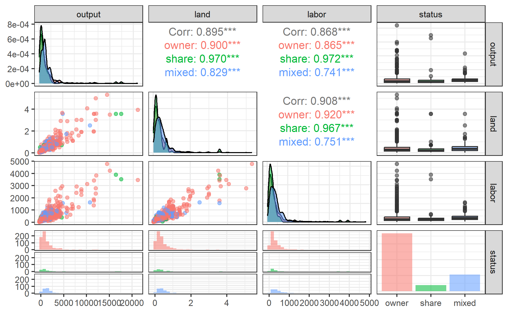
ggpairs(farm_dta, aes(colour = status, alpha = 0.2))

Regression and interpretation

fit1 <- lm(output ~ status + land + labor, 
           data = farm_dta)

fit2_cd <- lm(log(output) ~ status + log(land) + log(labor), 
           data = farm_dta)

modelsummary(
  list(`Linear prod.fn. (level-level)` = fit1,
       `CD prod.fn. (log-log)` = fit2_cd),
  estimate = "{estimate} {stars} ({std.error})", 
  statistic = NULL
)
Linear prod.fn. (level-level) CD prod.fn. (log-log)
(Intercept) 6.203
(36.845)
5.703 ***
(0.202)
Sharecropping 87.849
(96.953)
0.004
(0.047)
Mixed -90.608
(63.901)
0.017
(0.031)
Land, ha 2145.659 ***
(111.521)
0.679 ***
(0.027)
Labor, hours 1.248 ***
(0.126)
0.344 ***
(0.030)
Num.Obs. 1026 1026
R2 0.819 0.843
R2 Adj. 0.819 0.842
F 1158.652 1369.377

Conclusion

Linear prod. fn. (level-level) CD prod. fn. (log-log)
(Intercept) 6.203
(36.845)
5.703 ***
(0.202)
Sharecropping 87.849
(96.953)
0.004
(0.047)
Mixed -90.608
(63.901)
0.017
(0.031)
Land, ha 2145.659 ***
(111.521)
0.679 ***
(0.027)
Labor, hours 1.248 ***
(0.126)
0.344 ***
(0.030)
Num.Obs. 1026 1026
R2 0.819 0.843
R2 Adj. 0.819 0.842
F 1158.652 1369.377
  • Interpret coefficients in both models.

  • What is the estimated effect of share-cropping?

  • Is this model shows causal effects of \(x\) on \(y\)?

  • Is there a ceteris paribus?

Entertainment: Fitted values (1)

farm_dta %>% 
  mutate(fitted = fitted(fit1)) %>% 
  ggplot() + 
  aes(x = land,
      y = output,
      colour = "Observed") +
  xlab("Land area, ha") + 
  ylab("Rice output, kg")

Entertainment: Fitted values (1)

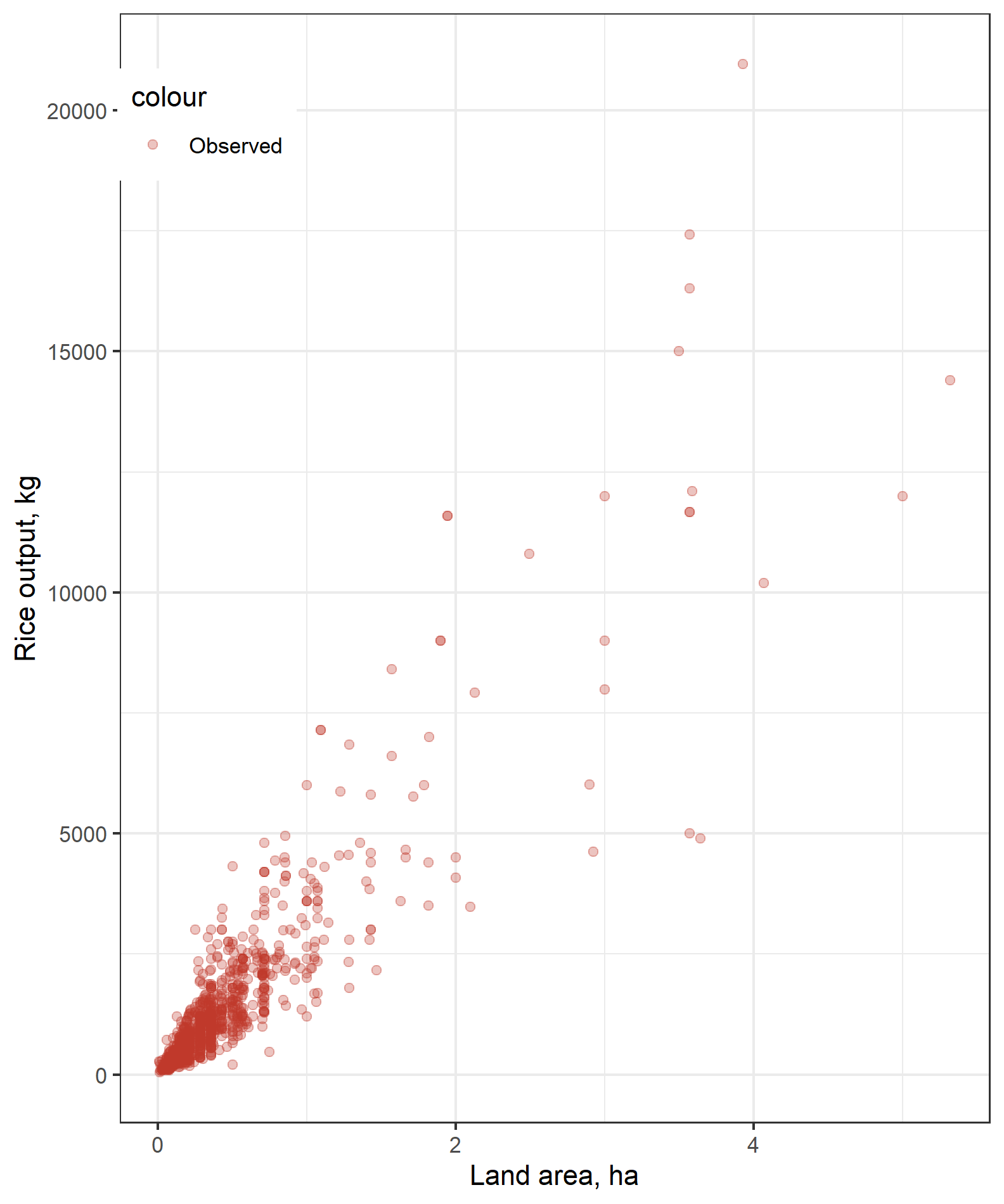
farm_dta %>% 
  mutate(fitted = fitted(fit1)) %>% 
  ggplot() + 
  aes(x = land,
      y = output,
      colour = "Observed") +
  xlab("Land area, ha") + 
  ylab("Rice output, kg") +
  geom_point(alpha = 0.3) + 
  theme(legend.position = c(0.1, 0.9)) + 
  scale_color_manual(
    values = c('#BF382A', '#0C4B8E'))

Entertainment: Fitted values (1)

farm_dta %>%
  mutate(fitted = fitted(fit1)) %>%
  ggplot() +
  aes(x = land,
      y = output,
      colour = "Observed") +
  xlab("Land area, ha") + 
  ylab("Rice output, kg") +
  geom_point(alpha = 0.3) +
  theme(legend.position = c(0.1, 0.9)) + 
  scale_color_manual(
    values = c('#BF382A', '#0C4B8E')) +
  geom_point(
    aes(y = fitted, colour = "Gitted"),
    alpha = 0.3)
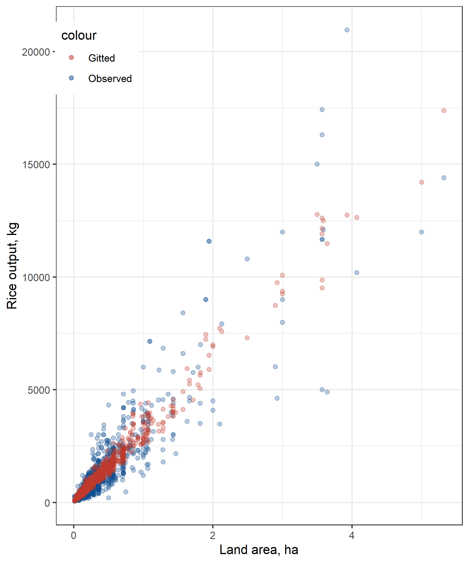
Entertainment: Fitted values (1)

farm_dta %>%
  mutate(fitted = fitted(fit1)) %>%
  ggplot() +
  aes(x = land,
      y = output,
      colour = "Observed") +
  xlab("Land area, ha") + 
  ylab("Rice output, kg") +
  geom_point(alpha = 0.3) +
  theme(legend.position = c(0.1, 0.9)) + 
  scale_color_manual(
    values = c('#BF382A', '#0C4B8E')) +
  geom_point(
    aes(y = fitted, colour = "Gitted"),
    alpha = 0.3) + 
  scale_x_log10() +
  scale_y_log10()
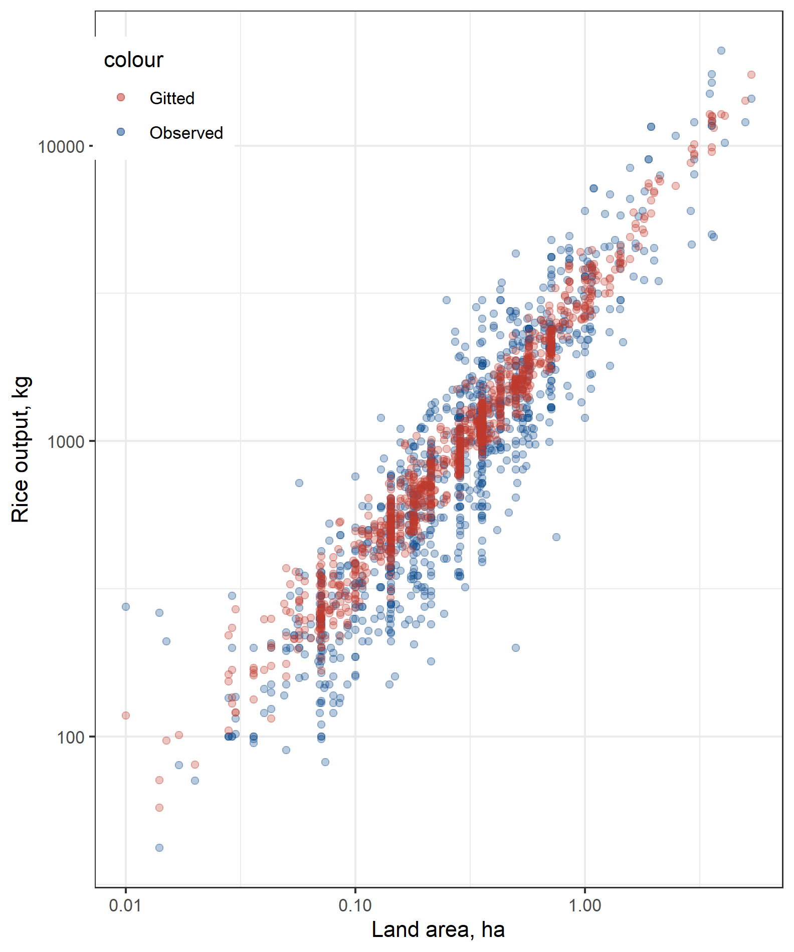
Entertainment: Actual values 3D

Entertainment: Actual + Fitted values 3D

Entertainment: Fitted values 3D v.2

Assumptions

  1. Linearity - validated using data

  2. Random sampling - “accepted based on faith in data collectors”

  3. No (Perfect) Collinearity - validated using data

  4. No Endogeneity - OVB

  5. Homoscedasticity (No heteroscedasticity) - validated using data

  6. Normality - validated using data

Linearity

Means: in \(y = \alpha + \beta x\); \(y\) is a linear function of \(x\).

If violated: \(\alpha\) and \(\beta\) are biased and inefficient.

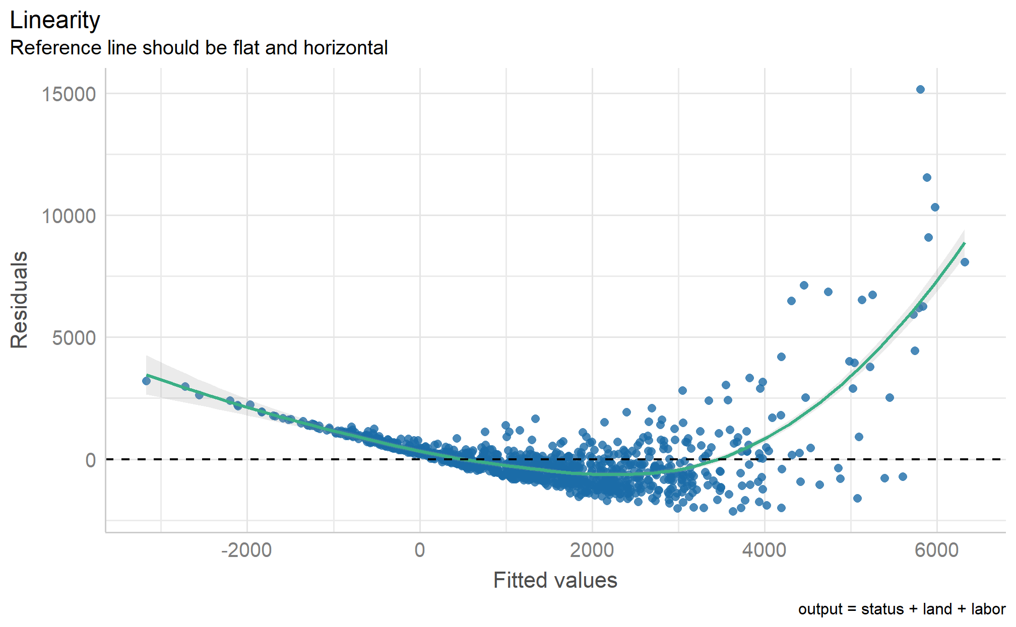
Detected: with scatter plots: \(y\) against \(x\), observed/residuals against fitted).

Resolved: with a linear transformation.

Linearity detection: scatter plots

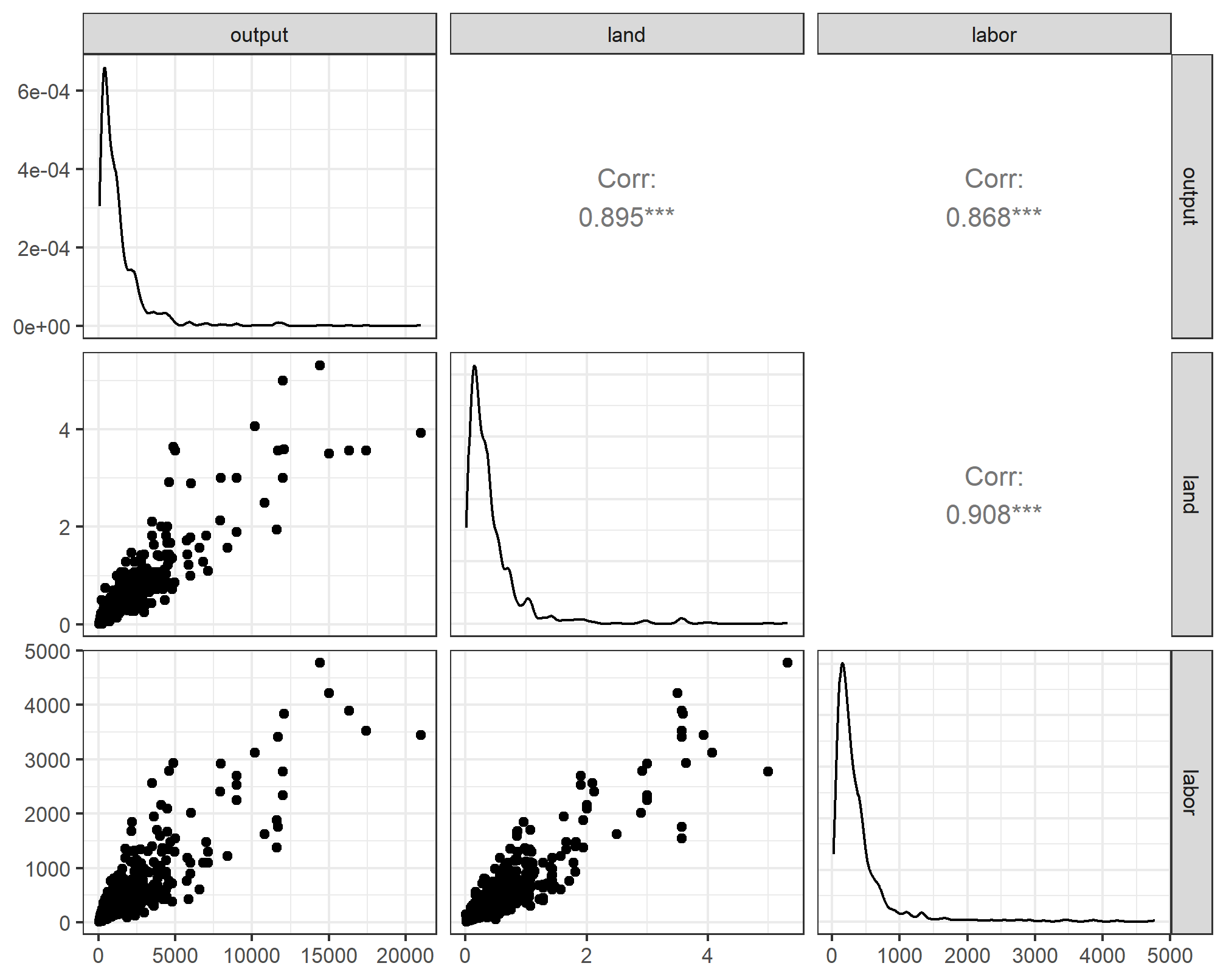
farm_dta %>% select(-status) %>% ggpairs()

  • Note the magnitude of \(x\) and \(y\)

  • From min to max \(y\) increases about 5000 times.

  • If a variable increases more than 10 times between min and max, \(log\) transformation may be needed.

Linearity detection: fitted values vs residuals
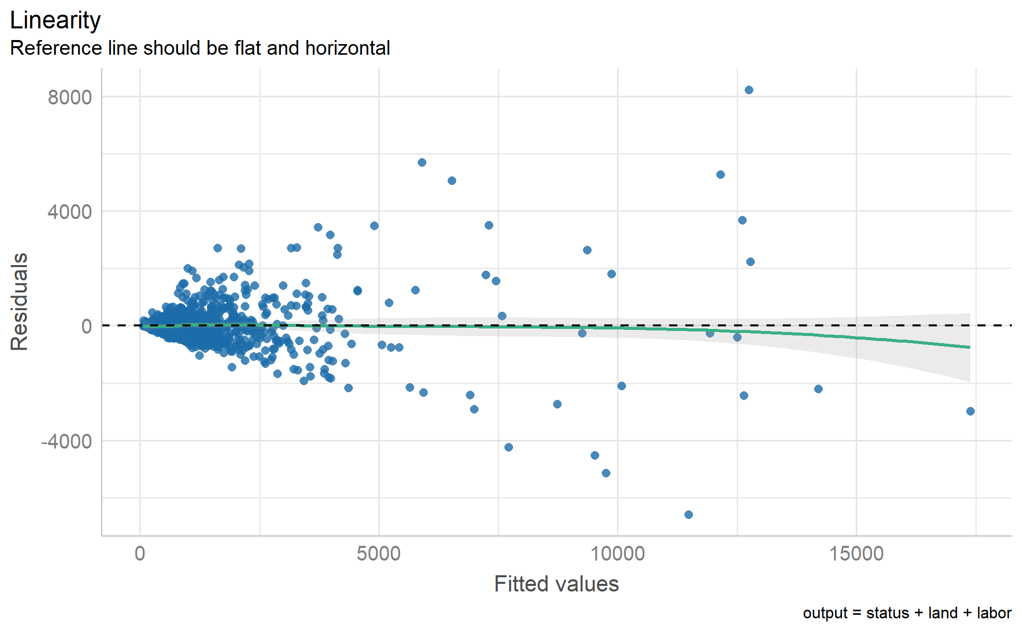
library(performance)
check_model(fit1, check = "linearity", panel = FALSE)

Linearity detection: fitted values vs residuals (v2)
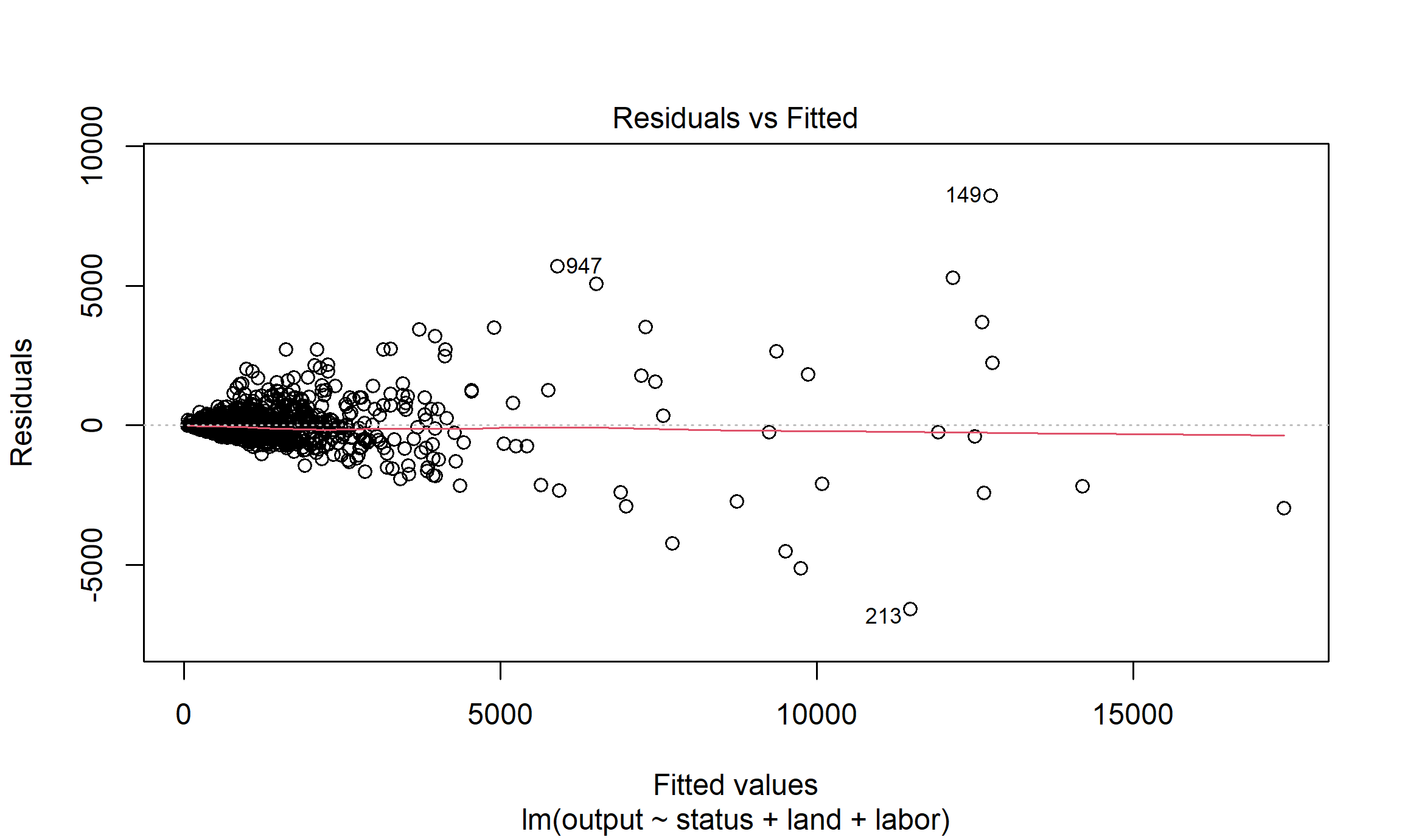
plot(fit1, which = 1)

Linearity Conclusion

Model:

lm(formula = output ~ status + land + labor, data = farm_dta)

Is the linearity assumption fulfilled?

What could be done to improve the model?

Linear transformation with log: partial (level-log or log-level) or full (log-log).

\[\ln (\text{output}) = \alpha + \beta_1 \text{status : share} + \beta_2 \text{status : mixed} \\ + \beta_3 \ln (\text{land}) + \beta_4 \ln (\text{labor}) + e\]

Linear transformation of the model

fit1 <- lm(output ~ status + land + labor, 
           data = farm_dta)

fit2_cd <- lm(output ~ status + log(land) + log(labor), 
           data = farm_dta)

modelsummary(
  list(`Linear prod.fn. (level-level)` = fit1,
       `CD prod.fn. (log-log)` = fit2_cd),
  estimate = "{estimate} {stars} ({std.error})", 
  statistic = NULL
)

Linear transformation of the model

Linear prod.fn. (level-level) CD prod.fn. (log-log)
(Intercept) 6.203 (36.845) 5.703 *** (0.202)
Sharecropping 87.849 (96.953) 0.004 (0.047)
Mixed -90.608 (63.901) 0.017 (0.031)
Land, ha 2145.659 *** (111.521) 0.679 *** (0.027)
Labor, hours 1.248 *** (0.126) 0.344 *** (0.030)
Num.Obs. 1026 1026
R2 0.819 0.843
R2 Adj. 0.819 0.842
F 1158.652 1369.377

Change in the linearity assumption

Without log-log
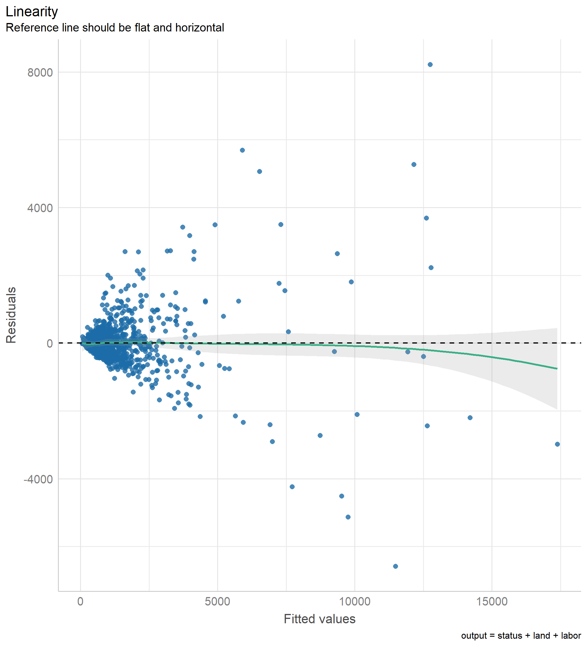
With log-log
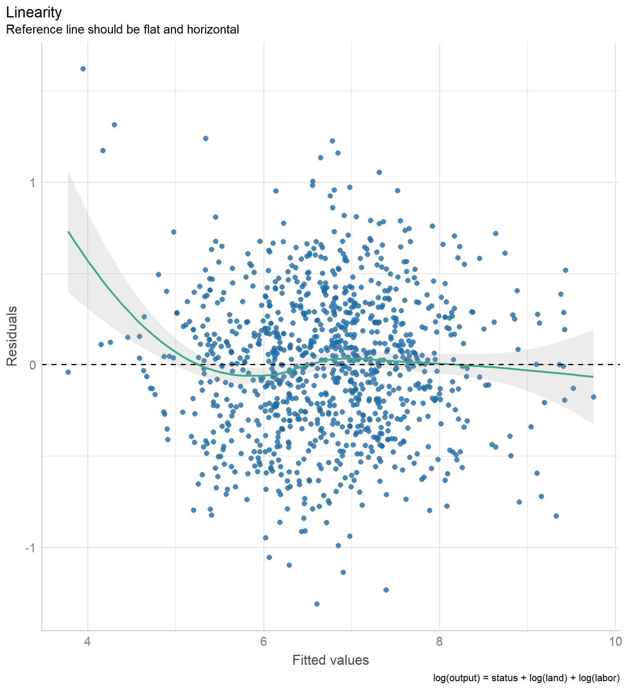
Change in Fitted values 3D v.2

Partial transformation (1)

fit3_level_log <- lm(output ~ status + log(land) + log(labor), data = farm_dta)
Linear prod.fn. (level-level) CD prod.fn. (log-log) Level-log prod.fn. (level-log)
(Intercept) 6.203 (36.845) 5.703 *** (0.202) -2549.390 *** (666.234)
Sharecropping 87.849 (96.953) 0.004 (0.047) 132.761 (154.889)
Mixed -90.608 (63.901) 0.017 (0.031) -480.042 *** (102.642)
Land, ha 2145.659 *** (111.521) 0.679 *** (0.027) 743.287 *** (89.588)
Labor, hours 1.248 *** (0.126) 0.344 *** (0.030) 901.025 *** (100.797)
Num.Obs. 1026 1026 1026
R2 0.819 0.843 0.540
R2 Adj. 0.819 0.842 0.538
F 1158.652 1369.377 299.783

Partial transformation (2)

check_model(fit3_level_log, check = "linearity", panel = FALSE)

No (perfect) collinearity (multicollinearity)

Two sub-problems:

  1. Perfect collinearity: when present regression will not be estimated.

  2. Near-perfect collinearity: regression works, but inference is misleading.

No Perfect Collinearity

Problem:

  • none of the regressors can be written as an exact linear combinations of some other regressors in the model.

  • For example:

    • in \(y = \beta_0 + \beta_1 x_1 + \beta_2 x_2 + \beta_3 x_3\) ,
    • where \(x_3 = x_2 + x_1\),
    • all \(x_i\) are collinear.

Detection: Through a regression equation

Solution: model re-specification.

Perfect Collinearity Example 1

\[ \begin{aligned} \hat{wage} & = \alpha + \hat\beta_1 education + \hat\beta_2 experience \\ & + \hat\beta_3 male + \hat\beta_4 female \end{aligned} \]

  • \(male + female = 1\)

  • Is there a multicollinearity problem here?

Perfect Collinearity Example 2

\[ \begin{aligned} \hat{output} & = \alpha + \hat\beta_1 land + \hat\beta_2 seeds + \hat\beta_3 fertilizers \\ & + \hat\beta_4 others + \hat\beta_5 total \end{aligned} \]

  • where \(total = seeds + fertilizers + others\)

  • Is there a multicollinearity problem here?

  • Coefficient \(\hat\beta_5\) is aliased and wont be estimated

Perfect Collinearity Example 3

Same model but in log:

\[ \begin{aligned} \ln (\hat{output})& = \hat\beta_1 \ln (land) + \hat\beta_2 \ln (seeds) + \hat\beta_3 \ln (fertilizers) \\ & + \hat\beta_4 \ln (others) + \hat\beta_5 \ln (total) \end{aligned} \]

where \(total = seeds + fertilizers + others\)

  • Is there a multicollinearity problem here?

  • Think!

  • \(log(a) + log(b) = log(a * b)\)

  • Danger

    No, there is no collinearity because \(\ln (seeds) + \ln (fertilizers) + \ln (others) \ne \ln (total)\). This is not a linear combination! \(\ln (seeds \cdot fertilizers \cdot others) \ne \ln (total)\)

Perfect Collinearity Example 4

Using the production function estimated above, let us convert tenure type into a set of dummy variables:

farm_dta_coll <- 
  farm_dta %>% 
  mutate(
    status_owner = ifelse(status == "owner", 1, 0),
    status_share = as.integer(status == "share"),
    status_mixed = as.integer(status == "mixed")
    )
glimpse(farm_dta_coll)
Rows: 1,026
Columns: 7
$ output       <int> 7980, 4083, 2650, 4500, 16300, 17424, 3840, 2800, 950, 24…
$ land         <dbl> 3.000, 2.000, 1.000, 2.000, 3.572, 3.572, 1.420, 1.420, 0…
$ labor        <int> 2915, 2155, 1075, 2091, 3889, 3519, 810, 855, 460, 109, 2…
$ status       <fct> owner, owner, owner, owner, share, share, mixed, mixed, m…
$ status_owner <dbl> 1, 1, 1, 1, 0, 0, 0, 0, 0, 1, 0, 0, 1, 1, 1, 0, 1, 1, 1, …
$ status_share <int> 0, 0, 0, 0, 1, 1, 0, 0, 0, 0, 1, 1, 0, 0, 0, 1, 0, 0, 0, …
$ status_mixed <int> 0, 0, 0, 0, 0, 0, 1, 1, 1, 0, 0, 0, 0, 0, 0, 0, 0, 0, 0, …

Perfect Collinearity Example 4


Call:
lm(formula = output ~ status_owner + status_share + status_mixed + 
    land + labor, data = farm_dta_coll)

Coefficients:
 (Intercept)  status_owner  status_share  status_mixed          land  
     -84.405        90.608       178.457            NA      2145.659  
       labor  
       1.248  

Call:
lm(formula = output ~ status_mixed + status_owner + status_share + 
    land + labor, data = farm_dta_coll)

Coefficients:
 (Intercept)  status_mixed  status_owner  status_share          land  
      94.052      -178.457       -87.849            NA      2145.659  
       labor  
       1.248  

Perfect Collinearity Example 4

Linear prod.fn. (level-level) Linear prod.fn. with dummies 1 Linear prod.fn. with dummies 2
(Intercept) 6.203 (36.845) -84.405 (60.186) 94.052 (93.612)
statusshare 87.849 (96.953)
statusmixed -90.608 (63.901)
land 2145.659 *** (111.521) 2145.659 *** (111.521) 2145.659 *** (111.521)
labor 1.248 *** (0.126) 1.248 *** (0.126) 1.248 *** (0.126)
status_owner 90.608 (63.901) -87.849 (96.953)
status_share 178.457 + (107.992)
status_mixed -178.457 + (107.992)
Num.Obs. 1026 1026 1026
R2 0.819 0.819 0.819
R2 Adj. 0.819 0.819 0.819
F 1158.652

Multicollinearity: Near-perfect collinearity

Problem

  • When two variables \(x_1\) and \(x_2\) are highly correlated.

  • And both (\(x_1\) and \(x_2\)) affect \(y\) significantly.

  • \(x_1\) and \(x_2\) are collinear

  • Estimated Standard Errors are inflated (larger then they could be).

  • Inference about \(x_1\) and \(x_2\) (only) is misleading.

Detection

  1. Variance Inflation Factor

    • Not a statistical test, only an informative number.
    • This shows by how much, the SE of the collinear variables are larger than what they could have been if there was no collinearity.
  2. Step-wise regression approach:

    • Include collinear variables one by one and together, and
    • observe how the \(R^2\), and variables significance changes

Solutions

  1. Find different independent variables.

  2. Drop one if it is redundant and repeating.

  3. Keep both and ignore if \(x_1\) and \(x_2\) are just control variables.

  4. Keep is removing may cause the OVB.

Multicollinearity Example 1. Production Function

library(performance)
check_collinearity(fit2_cd)
# Check for Multicollinearity

Low Correlation

       Term  VIF   VIF 95% CI Increased SE Tolerance Tolerance 95% CI
     status 1.02 [1.00, 1.49]         1.01      0.98     [0.67, 1.00]
  log(land) 4.36 [3.93, 4.87]         2.09      0.23     [0.21, 0.25]
 log(labor) 4.38 [3.94, 4.89]         2.09      0.23     [0.20, 0.25]

If VIF > 10, we may suspect multicollinearity.

Removing land or labor will cause the OVB (omitted variable bias), we must keep both variables.

Multicollinearity Example 2

\[ \begin{aligned} \hat{output} = \hat\beta_1 land + \hat\beta_2 seeds + \hat\beta_3 fertilizers + \hat\beta_4 others \end{aligned} \]

  • where \(seeds\) and \(fertilizers\) highly correlate between each other (r=0.9),

  • VIF of \(seeds\) and \(fertilizers\) is > 12.2

  • our key-interest variable is \(land\).

  • As \(fertilizers\) is a control variable and we may have OVB if we remove it,

  • If we really want to reduce VIF…:

    • Dis-aggregate fertilizers into mineral and organic, for example.
    • Aggregate fertilizers and seeds

Multicollinearity Example 3

Same model but with a quadratic term:

\[\hat{output} = \hat\beta_1 land + \hat\beta_2 land^2 + \hat\beta_3 seeds + \hat\beta_4 fertilizers + \hat\beta_5 others\]

  • VIF of \(land\) and \(land^2\) is > 25
  • Is there a multicollinearity problem here?
  • Think!
  • Not really
  • \(land^2\) is not a linear combination of \(land\) ;
  • Linear combination is when \(land + land\) not when \(land \times land\) ;

Multicollinearity Example 4

Step-wise approach to regression analysis:

Model 1 Model 2 Model 3 Model 4
(Intercept) 4.997*** (0.098) -20.158*** (2.726) -10.254*** (1.553) -1.278 (11.509)
muniPrecip -0.009+ (0.005) -0.010*** (0.002) -0.010*** (0.002) -0.011*** (0.002)
year 0.013*** (0.001) -0.011 (0.014)
log(muniPop) 1.025*** (0.104) 1.917 (1.138)
Num.Obs. 24 24 24 24
R2 0.148 0.832 0.848 0.852
R2 Adj. 0.110 0.815 0.833 0.830

Note: ^^ Model 1: log(muniUse) ~ muniPrecip
Model 2: log(muniUse) ~ muniPrecip + year
Model 3: log(muniUse) ~ muniPrecip + log(muniPop)
Model 4: log(muniUse) ~ muniPrecip + year + log(muniPop)

Homoscedasticity (No heteroscedasticity)

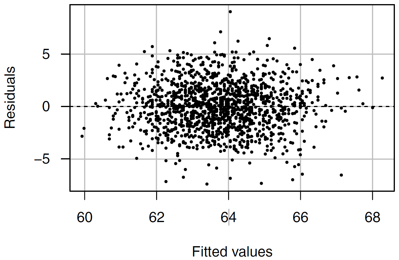
Homoscedasticity

\[ Var(u|x_{i1}, x_{i2}, \cdots , x_{ik}) = \sigma^2 \]
Problem and detection

  • Problem: when \(Var(u|x_{i1}, x_{i2}, \cdots , x_{ik}) \ne \sigma^2\)

    • Estimates are not biased, but;
    • Standard errors are inefficient;
    • Inference is misleading and false.
  • Detection:

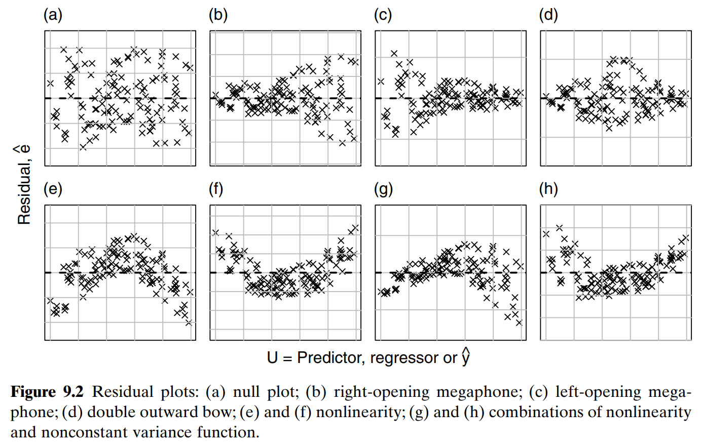
    • Graphical: residuals vs regressors and fitted values plots;
    • Statistical tests: Breusch-Pagan, White test, Goldfeld-Quandt.

Solutions

  • Re-specify the model/ choose different regressors;

  • Correct SE with alternative estimation procedures

    • robust: use heteroskedasticity-consistent (robust) standard errors.
    • cluster: use clustered standard errors.
  • Use a weighted regression estimated with Generalized Linear Model (GLM) estimator instead of OLS;

    • Generally discouraged for small samples (n < 5000) as GLM have weaker asymptotic properties as compared to the OLS.
  • See also: (Angrist & Pischke, 2009, Ch. 3.4), “Assumption AMLR.5” in (Wooldridge, 2020)

Heteroscedasticity example (1)

Heteroscedasticity (2). Production function

lm(formula = output ~ status + land + labor, data = farm_dta)
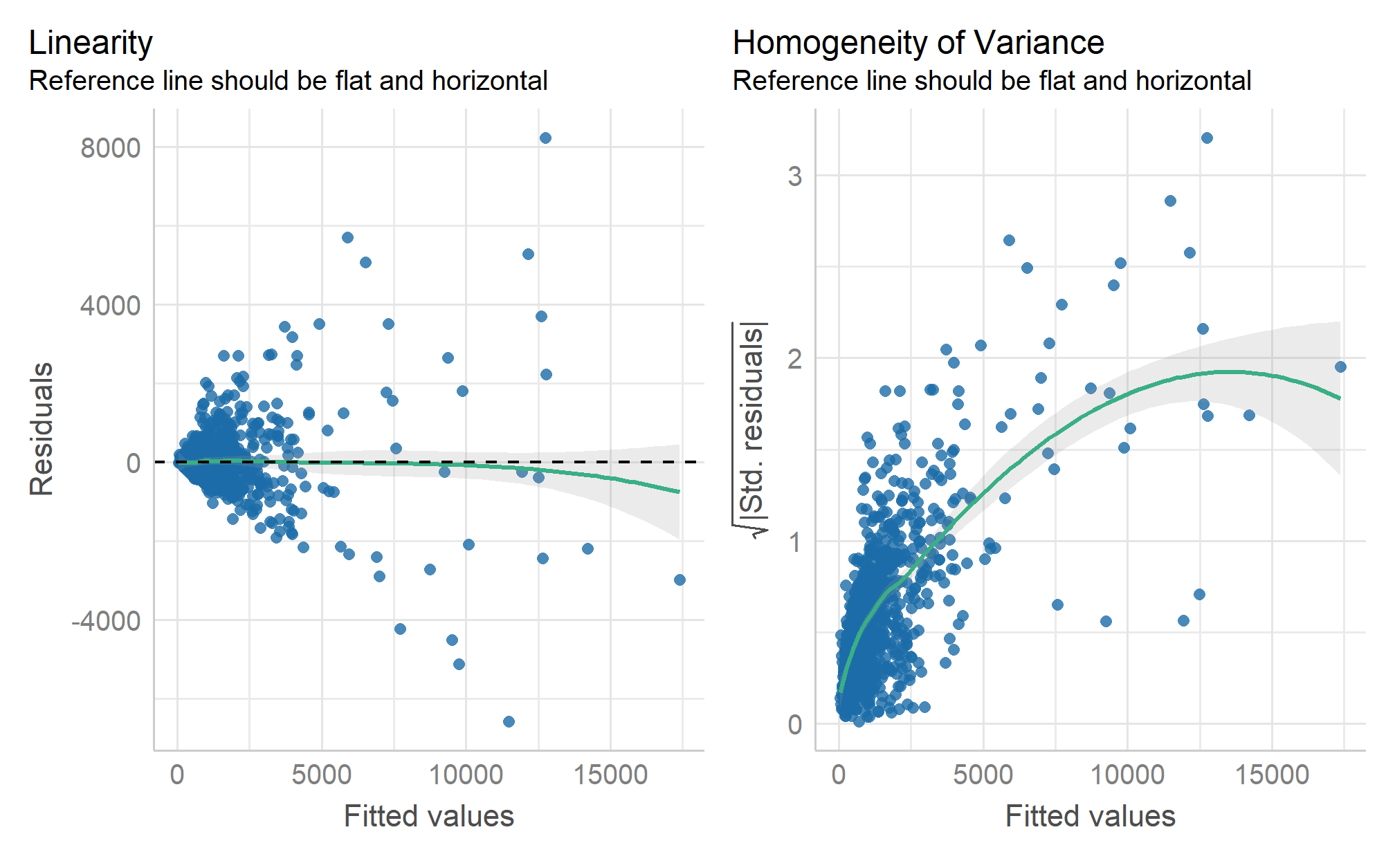
check_model(fit1, check = c("linearity", "homogeneity"))

Heteroscedasticity (2). Partial transformation

lm(formula = output ~ status + log(land) + log(labor), data = farm_dta)
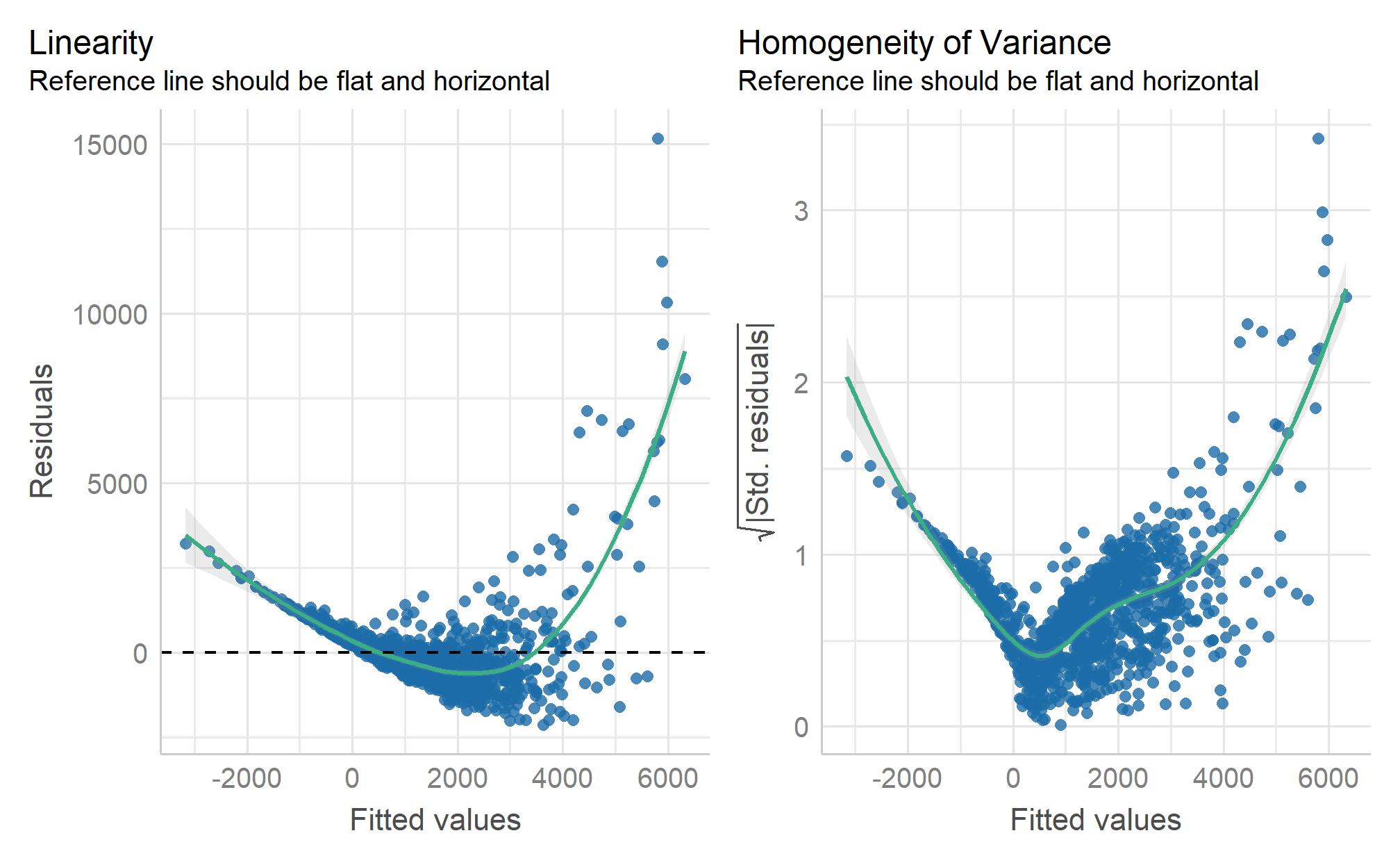
check_model(fit3_level_log, check = c("linearity", "homogeneity"))

Heteroscedasticity (2). CD production function

lm(formula = log(output) ~ status + log(land) + log(labor), data = farm_dta)
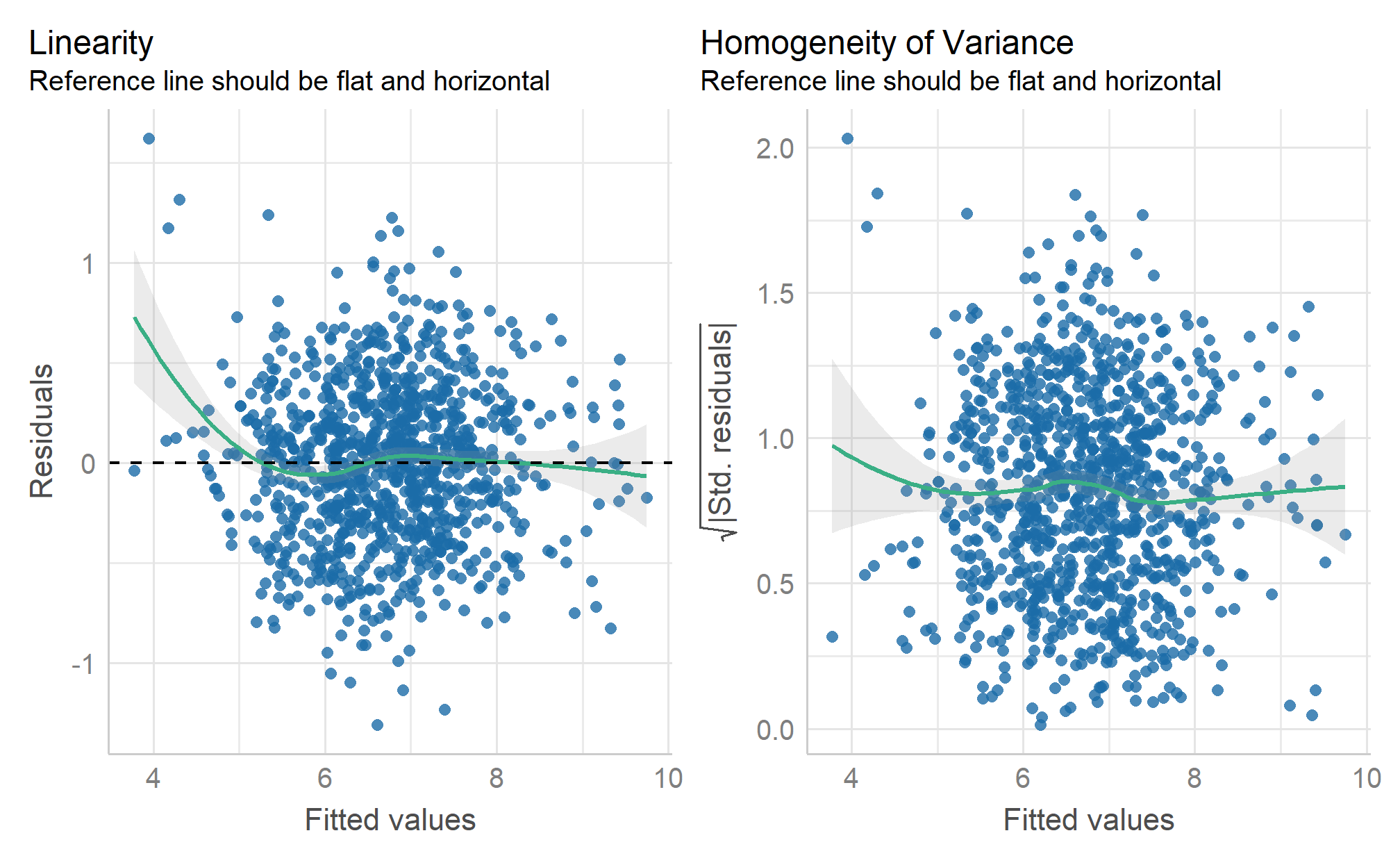
check_model(fit2_cd, check = c("linearity", "homogeneity"))

Statistical tests (1): Breusch-Pagan

  • \(H_0:\) variance is constant; \(H_1\) non constant variance.
  • If \(H_0\) is rejected, we have a Heteroscedasticity.
lm(formula = output ~ status + land + labor, data = farm_dta)
library(lmtest)
bptest(fit1)

    studentized Breusch-Pagan test

data:  fit1
BP = 348.57, df = 4, p-value < 2.2e-16
lm(formula = log(output) ~ status + log(land) + log(labor), data = farm_dta)
library(lmtest)
bptest(fit2_cd)

    studentized Breusch-Pagan test

data:  fit2_cd
BP = 19.776, df = 4, p-value = 0.0005528

Statistical tests (2): White test

Same idea as Breusch-Pagan test. Assumes that residuals variance is a function of polynomial of regressors:

\[ \text{residuals} = \log(\text{land}) + \log(\text{labor}) + \log(\text{land}) ^ 2 + \log(\text{labor})^2 \]

lm(formula = output ~ status + land + labor, data = farm_dta)
bptest(fit1, 
       ~ land * labor + I(labor^2) + I(labor^2), 
       data = farm_dta)

    studentized Breusch-Pagan test

data:  fit1
BP = 364.4, df = 4, p-value < 2.2e-16
lm(formula = log(output) ~ status + log(land) + log(labor), data = farm_dta)
bptest(fit1, 
       ~ log(land) * log(labor) + 
         I(log(labor)^2) + I(log(labor)^2), 
       data = farm_dta)

    studentized Breusch-Pagan test

data:  fit1
BP = 309.24, df = 4, p-value < 2.2e-16

Robust standard errors (1)

Methods of correcting the variance-covariance matrix.

vcov(fit1)
(Intercept) statusshare statusmixed land labor
(Intercept) 1357.56 -997.12 -909.30 -383.44 -0.71
statusshare -997.12 9399.81 910.48 -15.30 0.24
statusmixed -909.30 910.48 4083.37 -146.28 0.16
land -383.44 -15.30 -146.28 12437.02 -12.75
labor -0.71 0.24 0.16 -12.75 0.02

Common methods of robust standard errors

Robust estimators for variance covariance matrix:

  • sandwich::vcovHC - heteroskedasticity consistent

  • sandwich::vcovCL - clustered SE

  • clubSandwich::vcovCR - clustered heteroskedasticity consistent SE

  • sandwich::vcovHAC - heteroskedasticity and autocorrelation consistent

  • Estimation methods:

An example of robust vcov

lm(formula = output ~ status + land + labor, data = farm_dta)

Regular vcov

vcov(fit1)
(Intercept) statusshare statusmixed land labor
(Intercept) 1357.56 -997.12 -909.30 -383.44 -0.71
statusshare -997.12 9399.81 910.48 -15.30 0.24
statusmixed -909.30 910.48 4083.37 -146.28 0.16
land -383.44 -15.30 -146.28 12437.02 -12.75
labor -0.71 0.24 0.16 -12.75 0.02

Robust vcov

library(sandwich)
vcovHC(fit1, type = "HC3")
(Intercept) statusshare statusmixed land labor
(Intercept) 4235.06 -3084.98 249.07 -6038.87 -5.91
statusshare -3084.98 11437.98 799.53 -2421.05 8.76
statusmixed 249.07 799.53 2692.17 1349.86 -4.71
land -6038.87 -2421.05 1349.86 75901.71 -62.24
labor -5.91 8.76 -4.71 -62.24 0.09

Effect of robust SE on inference

lm(formula = output ~ status + land + labor, data = farm_dta)
Linear prod.fn. (level-level) regular SE
(Intercept) 6.203
(36.845)
Sharecropping 87.849
(96.953)
Mixed -90.608
(63.901)
Land, ha 2145.659 ***
(111.521)
Labor, hours 1.248 ***
(0.126)
Num.Obs. 1026
R2 Adj. 0.819
Linear prod.fn. (level-level) robust SE
(Intercept) 6.203
(68.312)
Sharecropping 87.849
(111.881)
Mixed -90.608 +
(53.100)
Land, ha 2145.659 ***
(291.480)
Labor, hours 1.248 ***
(0.312)
Num.Obs. 1026
R2 Adj. 0.819
Std.Errors HC3

Effect of robust SE on inference

lm(formula = log(output) ~ status + log(land) + log(labor), data = farm_dta)
CD prod.fn. (level-level) regular SE
(Intercept) 5.703 ***
(0.202)
Sharecropping 0.004
(0.047)
Mixed 0.017
(0.031)
Land, ha 0.679 ***
(0.027)
Labor, hours 0.344 ***
(0.030)
Num.Obs. 1026
R2 Adj. 0.842
CD prod.fn. (level-level) robust SE
(Intercept) 5.703 ***
(0.263)
Sharecropping 0.004
(0.048)
Mixed 0.017
(0.028)
Land, ha 0.679 ***
(0.036)
Labor, hours 0.344 ***
(0.039)
Num.Obs. 1026
R2 Adj. 0.842
Std.Errors HC3

Homework

Watch:

Reproduce analysis from the slides in R.

  • Make complex production function exercise.

Takeaways

  1. Assumptions and how to validated them.

  2. Statistical plots, measures (VIF), statistical tests and how to interpret them.

References

References

Angrist, J. D., & Pischke, J.-S. (2009). Mostly harmless econometrics. Princeton University Press. http://doi.org/10.1515/9781400829828
Dasgupta, S., Knight, T. O., & Love, H. A. (1999). Evolution of Agricultural Land Leasing Models: A Survey of the Literature. Applied Economic Perspectives and Policy, 21(1), 148–176. http://doi.org/10.2307/1349978
Feng, Q., & Horrace, W. C. (2010). Alternative technical efficiency measures: Skew, bias and scale. Journal of Applied Econometrics, 27(2), 253–268. http://doi.org/10.1002/jae.1190
Long, J. S., & Ervin, L. H. (2000). Using heteroscedasticity consistent standard errors in the linear regression model. The American Statistician, 54(3), 217–224. http://doi.org/10.1080/00031305.2000.10474549
Sadoulet, E., & de Janvry, A. (1995). Quantitative Development Policy Analysis. THE JOHNS HOPKINS UNIVERSITY PRESS BALTIMORE AND LONDON.
Wooldridge, J. M. (2020). Introductory econometrics: A modern approach. South-Western. Retrieved from https://www.cengage.uk/shop/isbn/9781337558860