Eduard Bukin
Fill in page 1 here: bit.ly/41R1YpL
Fill in page 2 here: bit.ly/41R1YpL
We do not make regression equations because we like how they look.
We base them on theory:
Here is one of many examples: Hedonic Model
To understand where the regression equation comes from, let us follow an example of:
Hedonic prices is an econometric approach of quantifying monetary values of differentiated characteristics (\(x_i\)) of goods and services, which are subjects of economic exchange (and stochastic variation \(u\)).
\[ \text{Price} = f(x_1, x_2, \cdots , x_i, u) \]
For example, agricultural land has such characteristics as: …
Land quality (location, slope, soil salinity, nutrient content, irrigation availability, rainfall, climate) environmental limitation, farmers’ accessibility, and other.
Hedonic equation is based on the theory that takes its roots to supply and demand.
Demand function:
\[Q_{t}^D = \alpha_0 + \alpha_1 P_t + u_{1t}, \;\; \text{with} \; \alpha_1 < 0\]
Supply function:
\[Q_{t}^S = \beta_0 + \beta_1 P_t + u_{2t}, \;\; \text{with} \; \beta_1 >0\]
Equilibrium condition:
\[ Q_{t}^S = Q_{t}^D \]
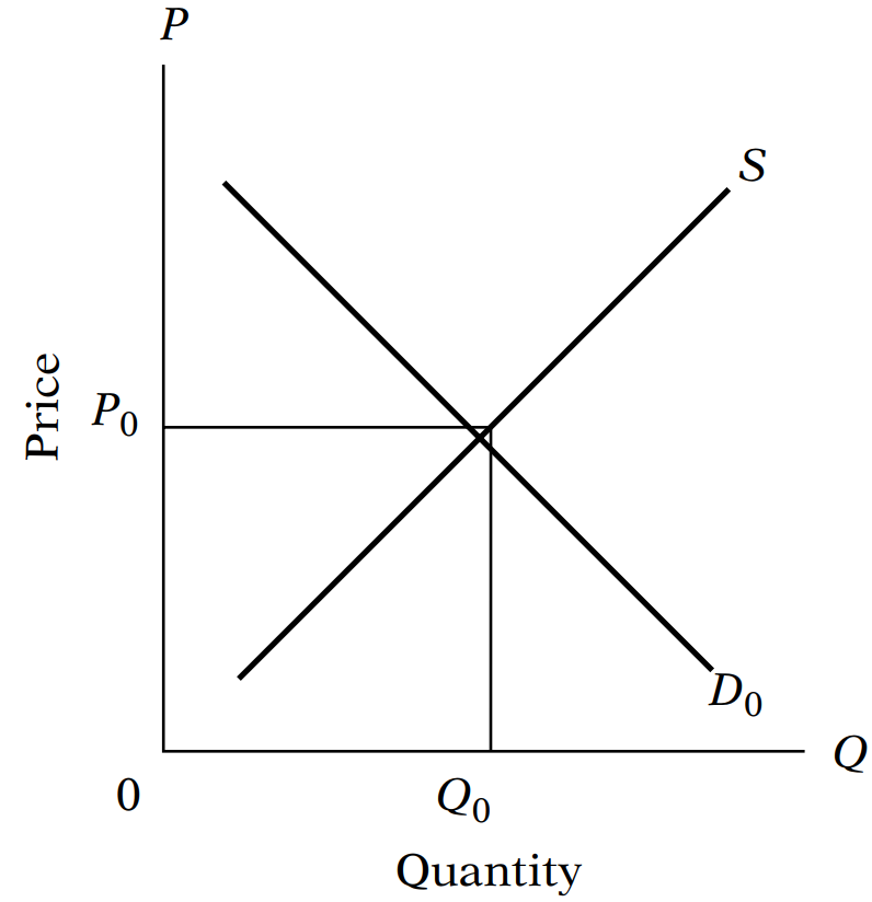
Relies on the partial equilibrium framework (Palmquist, 1989), where
Supply
\[ \phi(\hat{z}, \tilde{z}, \pi^{S^{'}}, r, \beta) \]
\(\hat{z}\) - land characteristics exogenous to land owner;
\(\tilde{z}\) - land characteristics in control of land owner;
Demand
\[ \pi^{S^{'}} + C(\hat{z}, \tilde{z}, r, \beta) \]
\(r\) - inputs prices;
\(\beta\) - technologies and opportunities such as credit availability;
\(\pi^{S^{'}}\) - expected profit of agricultural producers from land;
Supply-demand equilibrium:
\[\phi(\hat{z}, \tilde{z}, \pi^{S^{'}}, r, \beta) = R = \pi^{S^{'}} + C(\hat{z}, \tilde{z}, r, \beta)\]
Observed prices \(R\) are the equilibrium between bid and offer (demand and supply).
To explain causes behind price changes, we can deconstruct structural model into reduced form equations, which can be estimated:
Reduced form supply side
\[ R = \phi(\hat{z}, \tilde{z}, \pi^{S^{'}}, r, \beta) + e \]
Reduced form demand side
\[ R = \pi^{S^{'}} + C(\hat{z}, \tilde{z}, r, \beta) + e \]
When we run a hedonic prices model
\[R = R(\hat{z}, \tilde{z}, \pi^{S^{'}}, r, \beta)\]
we estimate one of the reduced forms and select independent variables based on the hedonic prices theory (differentiated land qualities).
\[R = R(\hat{z}, \tilde{z}, \pi^{S^{'}}, r, \beta)\]
Theory specifies key determinants of the outcome:
In \(R = R(\hat{z}, \tilde{z}, \pi^{S^{'}}, r, \beta)\), what are these independent and dependent variables?
03c-hedonic-land-prices.Rmd.We would like to assess the effect of the “Conservation Reserve Program” (CPR) on the agricultural land prices in Minnesota in 2002-2011.
Conservation Reserve Program
\[ \log (\text{acrePrice}) = \beta_0 + \beta_1 \text{crpPct} + \log(\beta_2 \text{acres}) + \beta_3 \text{region} \\ + \beta_4 \text{year} + \beta_4 \text{tillable} + \beta_5 \text{productivity} + \beta_6 \text{improvements} + e \]
acrePrice - sale price in dollars per acre;acres - size of the farm in acres;region - region in the state Minnesota;year - year of the land sales translation;crpPct - the percentage of all farm acres enrolled in CRP;tillable - percentage of farm acreage that is rated arable by the assessor;productivity - average agronomic productivity scaled 1 to 100, with larger numbers for more productive land;improvements - percentage of property value due to improvements (infrastructure)| log(Price per acre) | log(Price per acre) | |
|---|---|---|
| Intercept | 6.099 *** (0.051) | 6.507 *** (0.034) |
| Subsidy (0|1) | -0.00370 *** (0.00027) | -0.00488 *** (0.00017) |
| Area (log), acres | -0.0587 *** (0.0058) | -0.0913 *** (0.0051) |
| Tillable area, % (0-100) | 0.00421 *** (0.00036) | 0.00550 *** (0.00018) |
| Improvements, (0-100) | 0.01567 *** (0.00062) | 0.01414 *** (0.00033) |
| Productivity, (0-100) | 0.0094 *** (0.0004) | |
| West Central (0|1) | 0.633 *** (0.016) | 0.746 *** (0.011) |
| Central (0|1) | 0.885 *** (0.018) | 1.041 *** (0.013) |
| South West (0|1) | 0.734 *** (0.016) | 1.019 *** (0.011) |
| South Central (0|1) | 0.854 *** (0.017) | 1.191 *** (0.011) |
| South East (0|1) | 0.897 *** (0.018) | 1.234 *** (0.012) |
| Num.Obs. | 8770 | 17441 |
| R2 Adj. | 0.700 | 0.646 |
Note: ^^ Year-specific dummy variables are omitted. Heteroscedasticity consistent standard errors are reported in parentheses. P-values are coded as: * p=0.05, ** p=0.01, *** p<0.001
Shows the share of variance explained by a model adjusted to the number of independent variables.
If the number of independent variables increases, but variables do not explain \(y\) better, \(R^2\) adjusted could shrink to 0 or a negative number.
We generally want to have it as high as possible, however!
\(R^2\) adjusted has nothing to do with the coefficients’ significance and their causal meaning.
If the goal of regression is to explain causes, rather than predict outcomes, \(R^2\) adjusted has not much relevance.
Base on (Ashenfelter, Ashmore, & Lalonde, 1995)
What makes wine so expensive?
Any guesses?
Weather
Any unobserved characteristics?
\[ Price = \beta_0 + \beta_1 \text{Age} + \beta_2 \text{AGST} + \beta_3 \text{HarvestRain} + \beta_4 \text{WinterRain} + e \]
What are our expectations about signs of \(\beta\) s?
Price: average market price for Bordeaux vintages according to a series of auctions (USD). The price is relative to the price of the 1961 vintage, regarded as the best one ever recorded.WinterRain: winter rainfall (in mm).AGST: Average Growing Season Temperature (in Celsius degrees).HarvestRain: harvest rainfall (in mm).Age: age of the wine, measured in 1983 as the number of years stored in a cask.Exercise:
03-wine-regression.Rmd
“Regression is the tool that masters pick up first, if only to provide a benchmark for more elaborate empirical strategies.” (Angrist & Pischke, 2014)
“… regression estimates are weighted averages of multiple matched comparisons of the sort constructed for the groups in our stylized matching matrix.” (Angrist & Pischke, 2014)
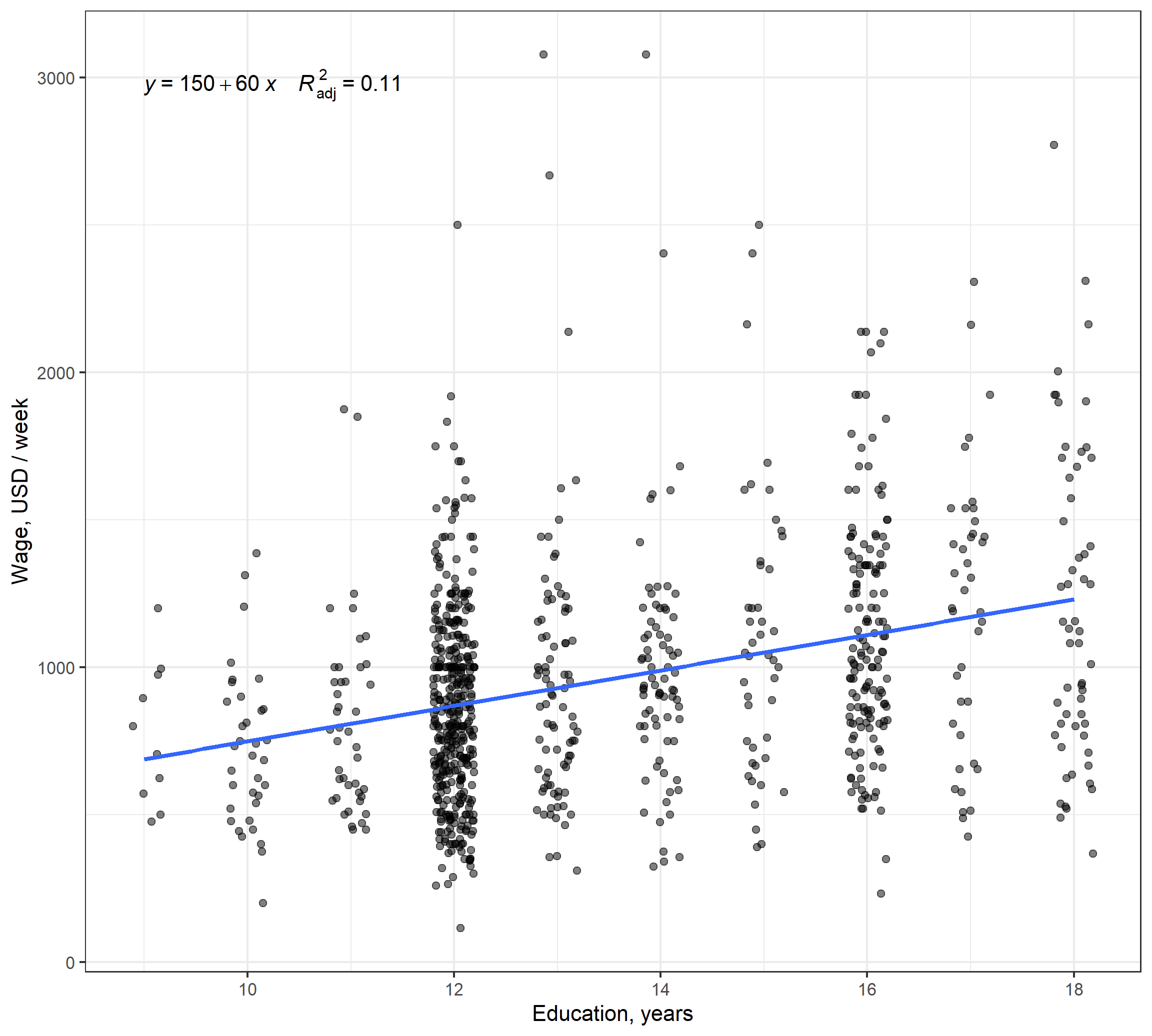
\[ Y_i = \alpha + \beta \, P_i + e_i, \]
where:
\(Y_i\) is wage in Euro per week
\(P_i\) is education in years
\(\alpha\) is the intercept
\(\beta\) is the slope or causal effect of interest
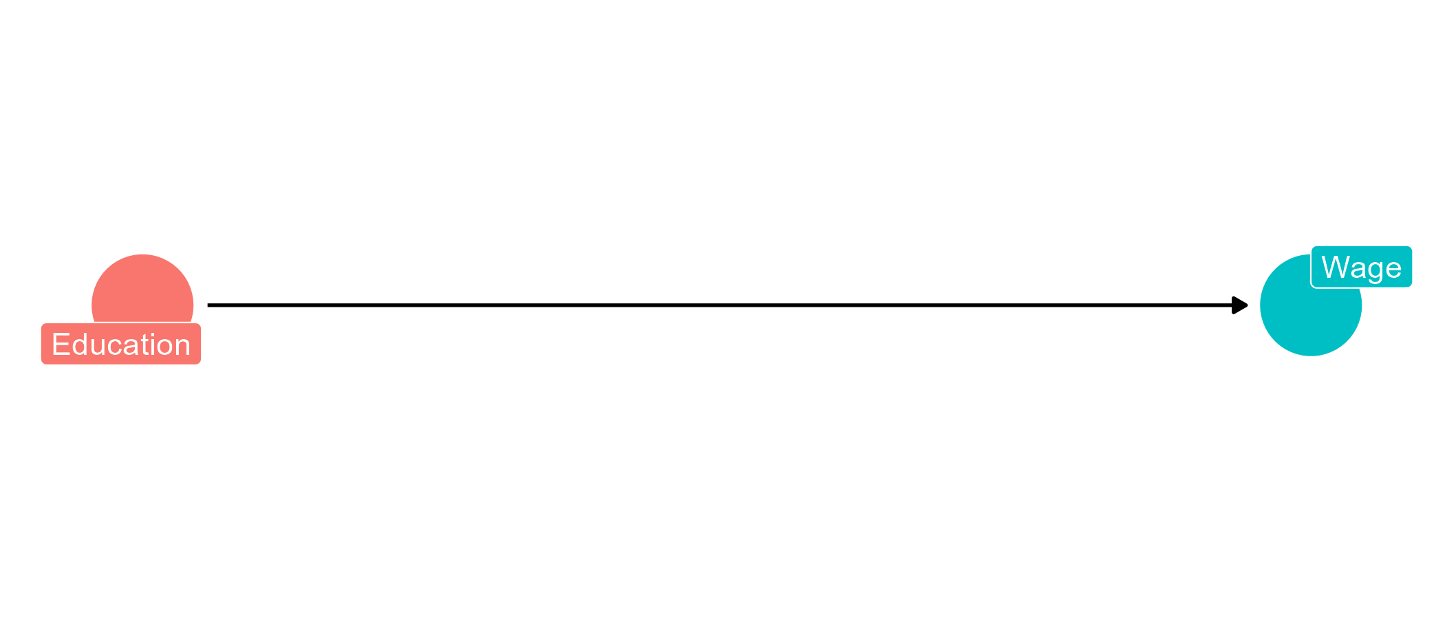
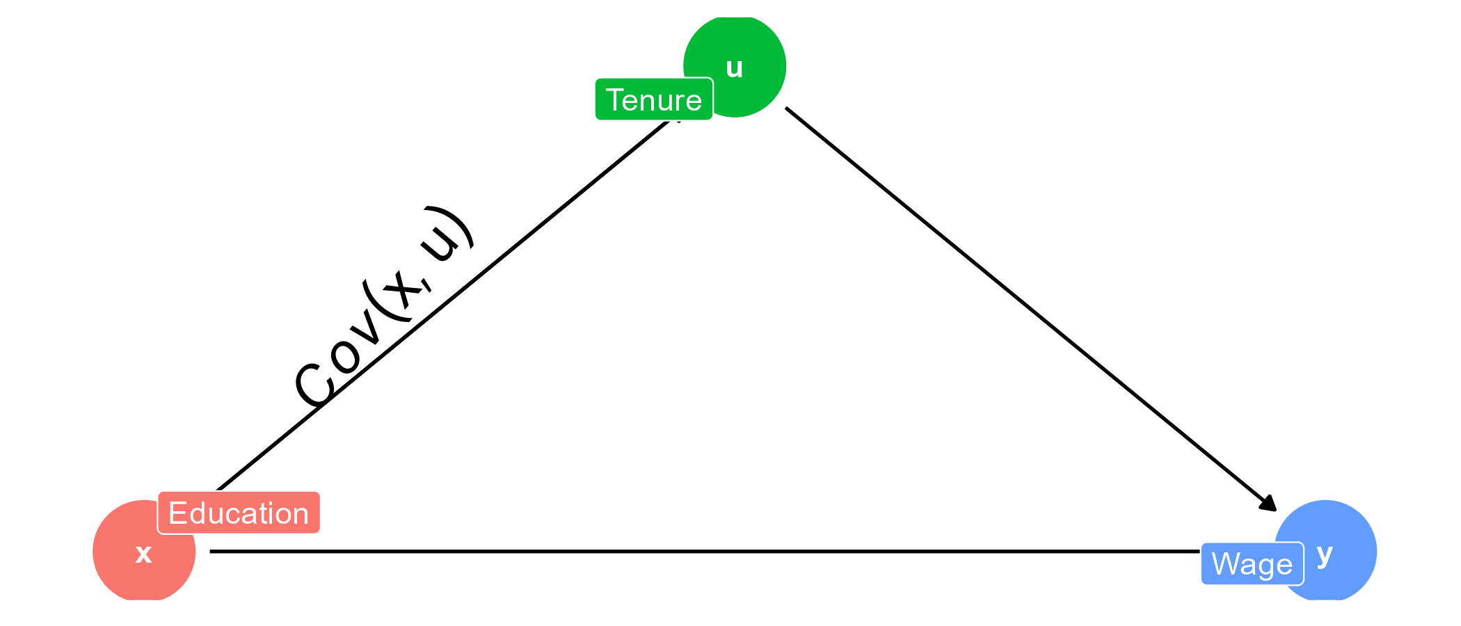
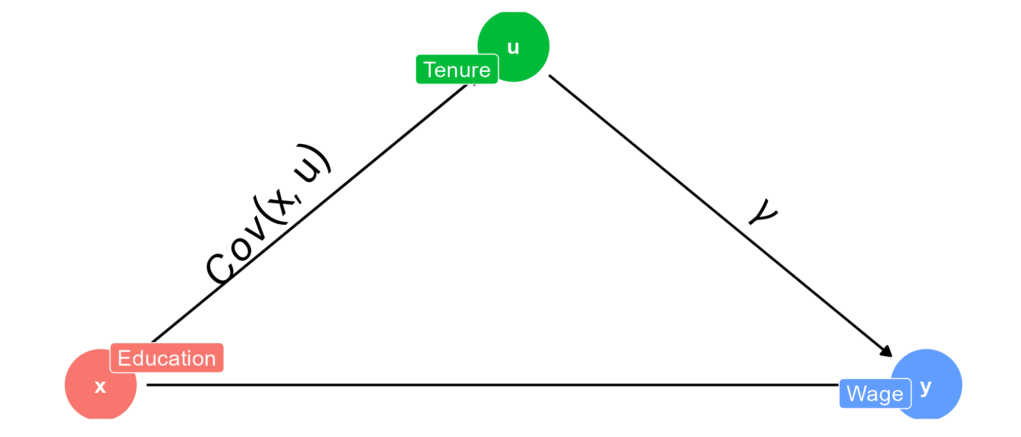
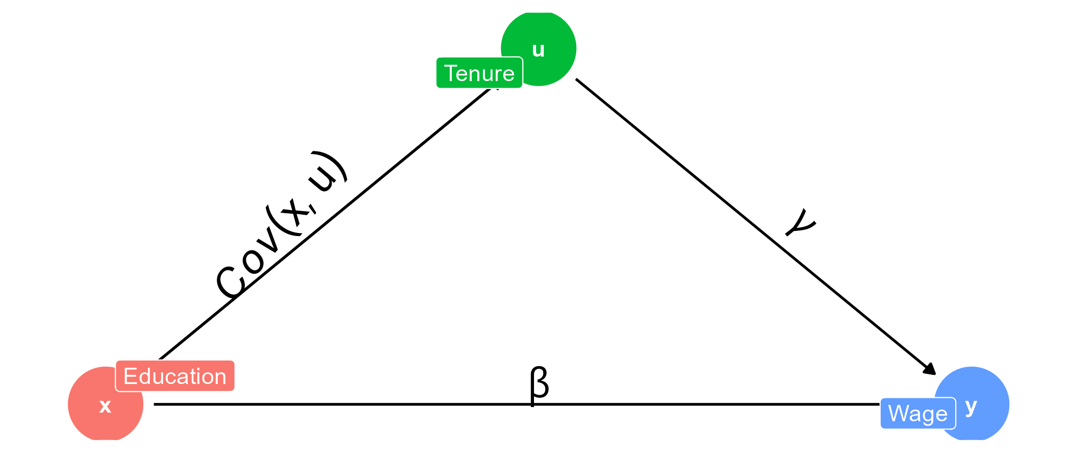
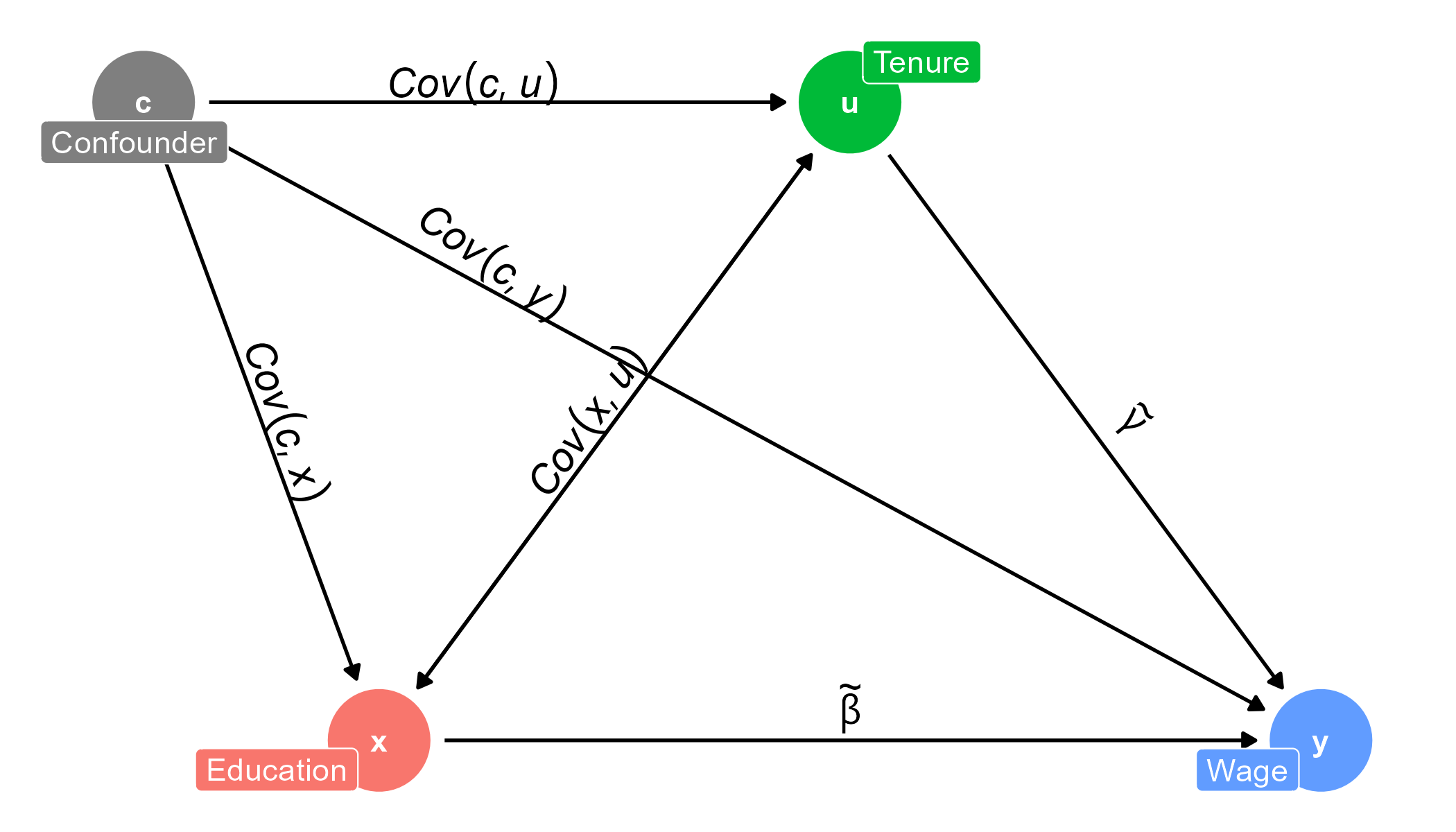
Causal directed acyclic graph.

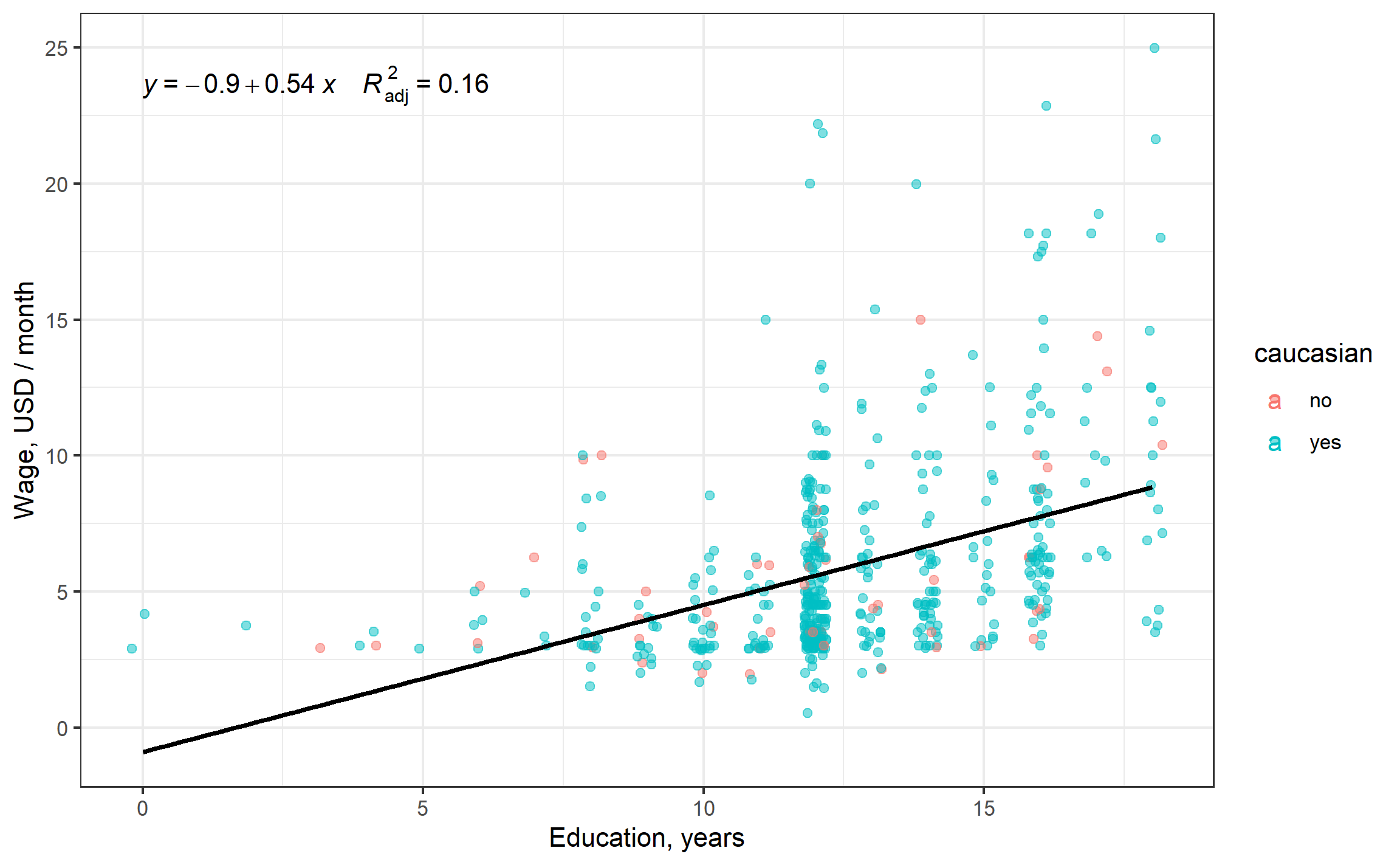
Interpret the effect of education on wage.
Is this a causal effect on education on wage?


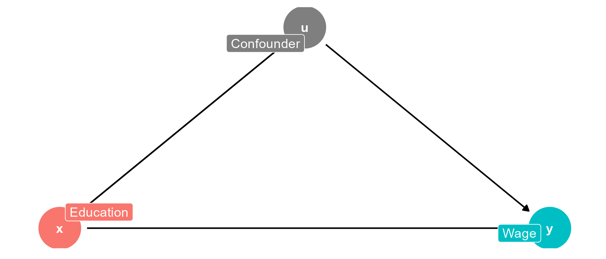
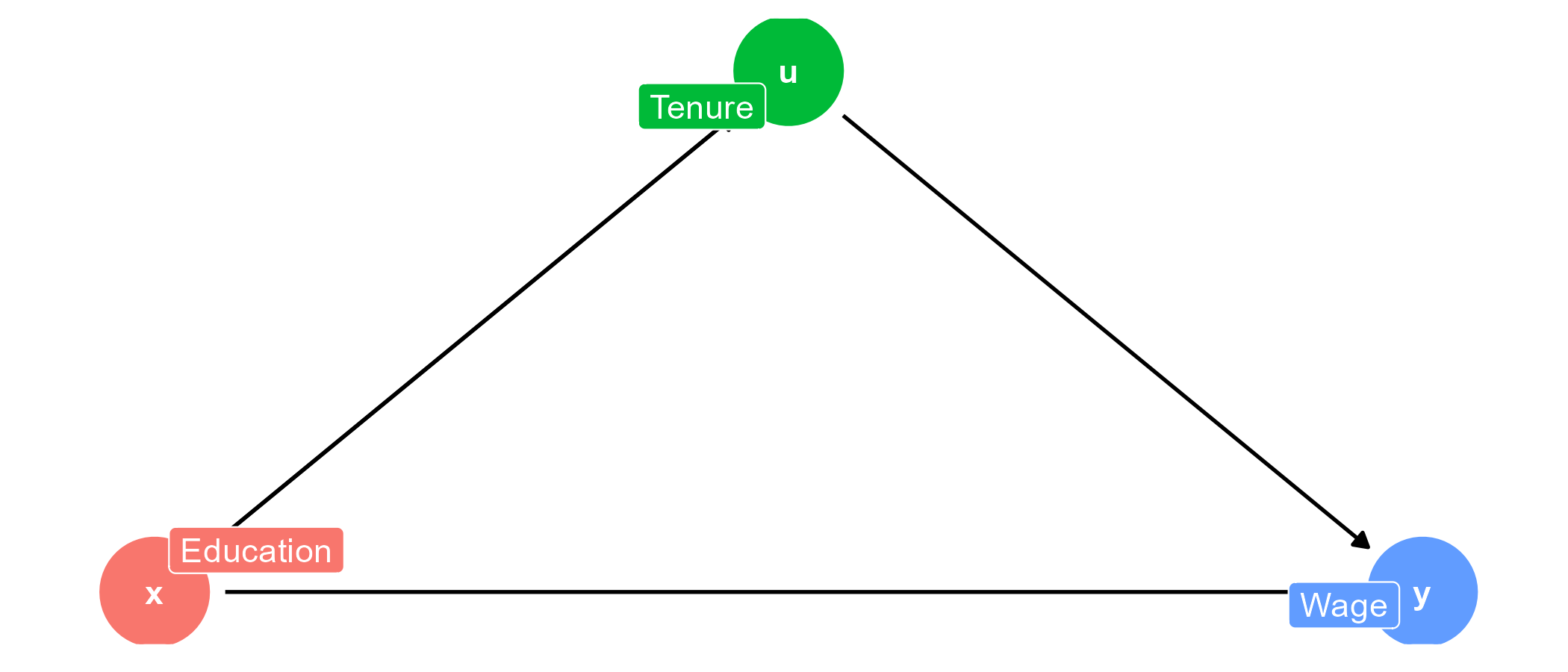
Regression accounts for the observed (included) confounders by attributing variance in \(y\) to the variance in \(x\) (variable of interest) and \(u\) (control variables).
\[ Y_i = \alpha + \beta \, P_i + \gamma \, A_i + e_i, \]
Regression controls the variance in \(Y_i\) with observed \(P_i\) and \(A_i\).
In the context of the variable of interest (\(P_i\)):
Regression controls other variables (\(A_i\)) fixed,
ensuring that \(\beta\) reviels causal effect Ceteris Paribus.


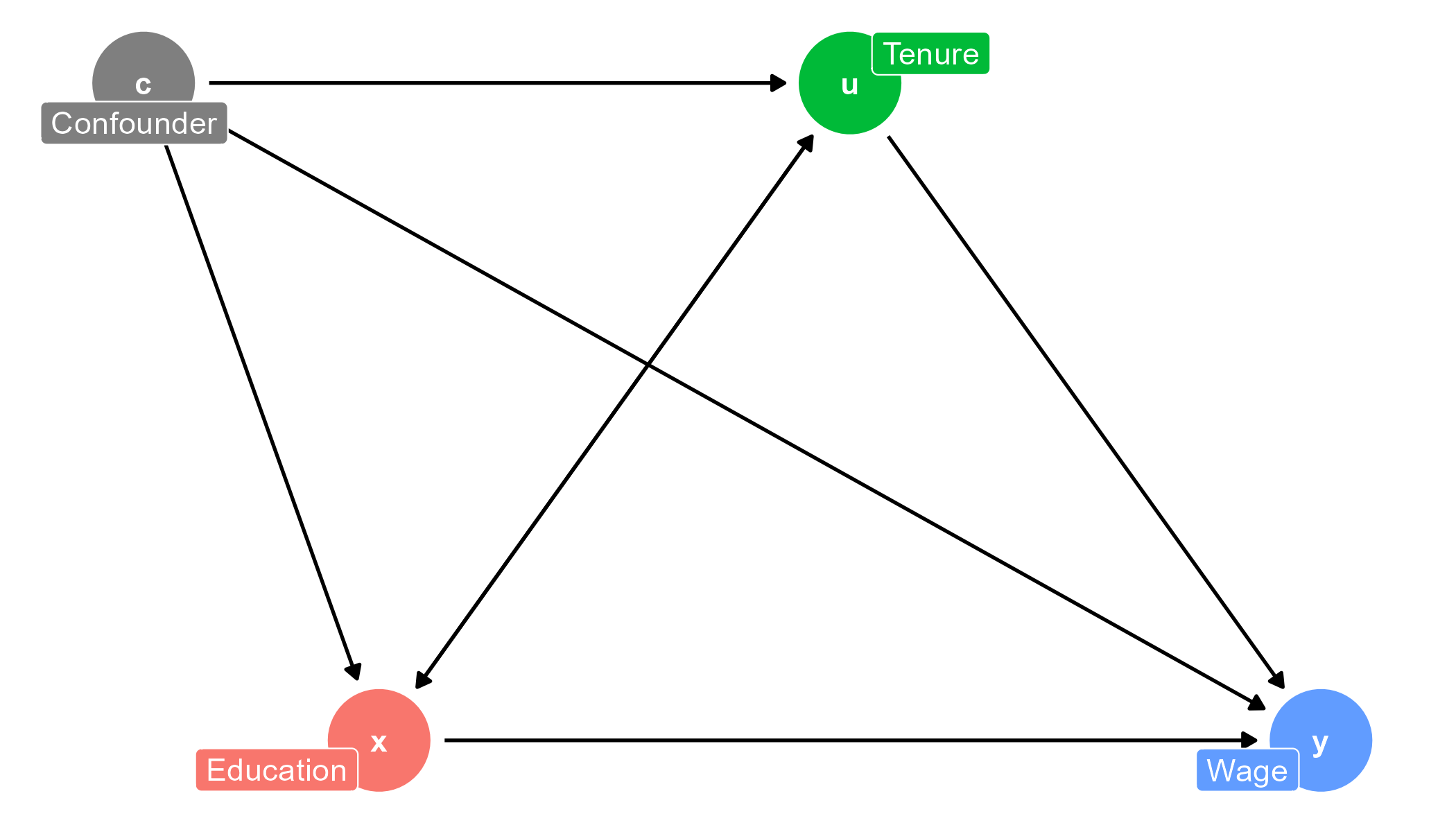
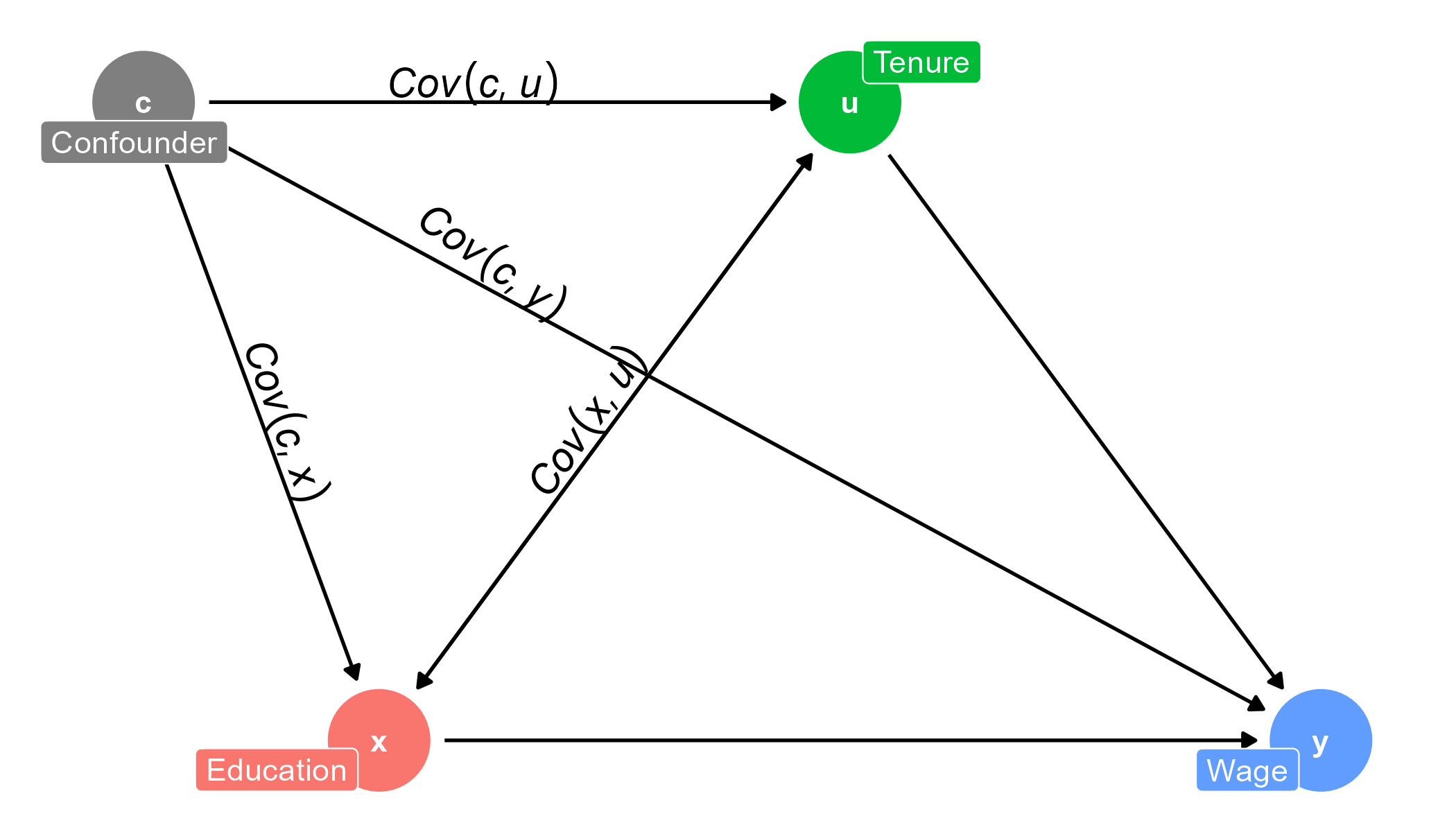
Not every confounded could be observed or measures.
There are unobserved ones:
When a confounded correlated with outcome \(Cov(c,y) \ne 0\) and other regressors \(Cov(c,u) \ne 0\) and \(Cov(c,x) \ne 0\).
Estimates of \(\beta\) and \(\gamma\) are no longer ceteris paribus!
Absence of the Ceteris Paribus in a regression is called omitted variable bias
Supposed that our ideal regression
\[ Y_i = \alpha ^ l + \beta ^ l P_i + \gamma A_i + e^l_i, \]
We cannot measure \(A_i\), but:
Because of the omitted variable,
we cannot estimate the long model.
Instead, we estimate a short model:
\[ Y_i = \alpha ^ s + \beta^s P_i + e^s_i \]
where omitted variable is implicit in the residuals:
\[ e^s_i = e^l_i + A_i \]
Omitted variable causes bias of all estimates!
This bias can be measured as \(\text{OVB}\):
\[ \text{OVB} = \beta^s - \beta^l \]
To be continued on the OVB in another week
Any ideas?
Any ideas?
We include control variables to reduce or defeat the omitted variable bias.
See Wooldridge (2020)
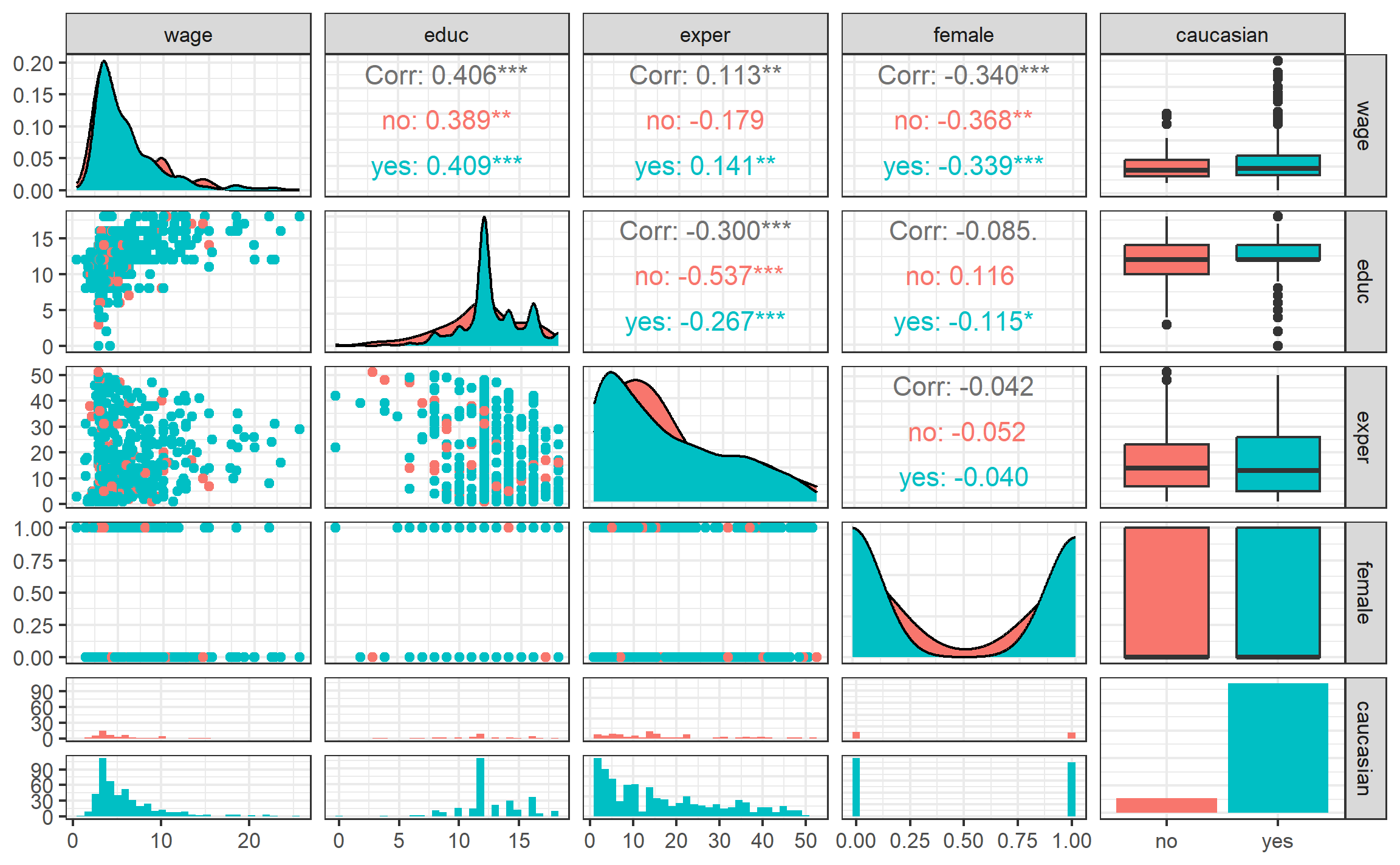
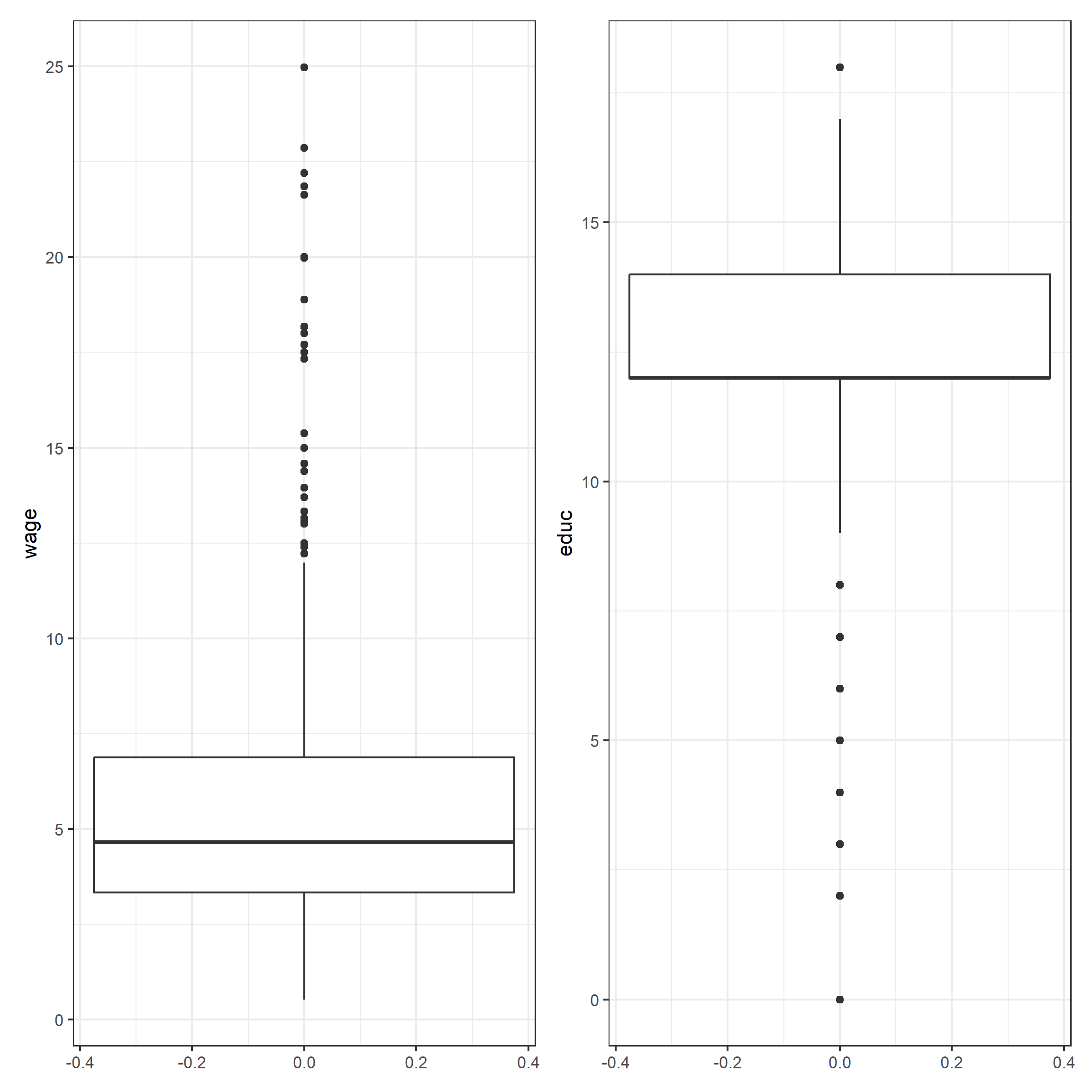
We use data from (Blackburn and Neumark, 1992) on wage determinants. Variables present are:
Our goal is to identify the causal effect of education on wage estimating following equation:
\[ \text{wage} = \beta_0 + \beta_1 \text{educ} + \beta_2 \text{exper} + \beta_3 \text{black} + \beta_4 \text{female} + e \]
Rows: 526
Columns: 7
$ wage <dbl> 3.10, 3.24, 3.00, 6.00, 5.30, 8.75, 11.25, 5.00, 3.60, 18.18…
$ educ <dbl> 11, 12, 11, 8, 12, 16, 18, 12, 12, 17, 16, 13, 12, 12, 12, 1…
$ exper <dbl> 2, 22, 2, 44, 7, 9, 15, 5, 26, 22, 8, 3, 15, 18, 31, 14, 10,…
$ black <dbl> 0, 0, 0, 0, 0, 0, 0, 0, 0, 0, 0, 0, 0, 0, 0, 0, 0, 0, 0, 0, …
$ white <dbl> 1, 1, 1, 1, 1, 1, 1, 1, 1, 1, 1, 1, 1, 1, 1, 1, 1, 1, 1, 1, …
$ female <dbl> 1, 1, 0, 0, 0, 0, 0, 1, 1, 0, 1, 1, 0, 0, 0, 0, 1, 1, 1, 1, …
$ caucasian <fct> yes, yes, yes, yes, yes, yes, yes, yes, yes, yes, yes, yes, …
| Unique (#) | Missing (%) | Mean | SD | Min | Median | Max | |
|---|---|---|---|---|---|---|---|
| wage | 241 | 0 | 5.9 | 3.7 | 0.5 | 4.7 | 25.0 |
| educ | 18 | 0 | 12.6 | 2.8 | 0.0 | 12.0 | 18.0 |
| exper | 51 | 0 | 17.0 | 13.6 | 1.0 | 13.5 | 51.0 |
| black | 2 | 0 | 0.1 | 0.3 | 0.0 | 0.0 | 1.0 |
| white | 2 | 0 | 0.9 | 0.3 | 0.0 | 1.0 | 1.0 |
| female | 2 | 0 | 0.5 | 0.5 | 0.0 | 0.0 | 1.0 |
Call:
lm(formula = wage ~ educ + exper + black + female, data = wage_dta)
Coefficients:
(Intercept) educ exper black female
-1.71453 0.60175 0.06422 -0.08389 -2.15649
Call:
lm(formula = wage ~ educ + exper + black + female, data = wage_dta)
Residuals:
Min 1Q Median 3Q Max
-6.3666 -1.9740 -0.4936 1.1248 14.8123
Coefficients:
Estimate Std. Error t value Pr(>|t|)
(Intercept) -1.71453 0.76169 -2.251 0.0248 *
educ 0.60175 0.05135 11.718 < 2e-16 ***
exper 0.06422 0.01041 6.168 1.39e-09 ***
black -0.08389 0.44430 -0.189 0.8503
female -2.15649 0.27060 -7.969 1.01e-14 ***
---
Signif. codes: 0 '***' 0.001 '**' 0.01 '*' 0.05 '.' 0.1 ' ' 1
Residual standard error: 3.081 on 521 degrees of freedom
Multiple R-squared: 0.3094, Adjusted R-squared: 0.304
F-statistic: 58.34 on 4 and 521 DF, p-value: < 2.2e-16
| Model 1 | |
|---|---|
| (Intercept) | -1.715 (0.762)* |
| educ | 0.602 (0.051)*** |
| exper | 0.064 (0.010)*** |
| black | -0.084 (0.444) |
| female | -2.156 (0.271)*** |
| Num.Obs. | 526 |
| R2 Adj. | 0.304 |
| F | 58.341 |
# Predicted values of wage
educ | Predicted | 95% CI
---------------------------------
0 | -1.66 | [-2.96, -0.37]
3 | 0.14 | [-0.86, 1.14]
5 | 1.35 | [ 0.54, 2.15]
7 | 2.55 | [ 1.93, 3.17]
10 | 4.35 | [ 3.99, 4.72]
12 | 5.56 | [ 5.29, 5.83]
14 | 6.76 | [ 6.46, 7.06]
18 | 9.17 | [ 8.56, 9.78]
Adjusted for:
* exper = 17.02
* black = 0.10
* female = 0.48
# Predicted values of wage
# female = 0
educ | Predicted | 95% CI
---------------------------------
0 | -0.63 | [-1.97, 0.71]
4 | 1.78 | [ 0.82, 2.74]
7 | 3.58 | [ 2.89, 4.27]
10 | 5.39 | [ 4.92, 5.85]
12 | 6.59 | [ 6.22, 6.96]
18 | 10.20 | [ 9.57, 10.84]
# female = 1
educ | Predicted | 95% CI
---------------------------------
0 | -2.79 | [-4.08, -1.49]
4 | -0.38 | [-1.30, 0.54]
7 | 1.43 | [ 0.77, 2.08]
10 | 3.23 | [ 2.79, 3.67]
12 | 4.43 | [ 4.05, 4.82]
18 | 8.04 | [ 7.35, 8.73]
Adjusted for:
* exper = 17.02
* black = 0.10
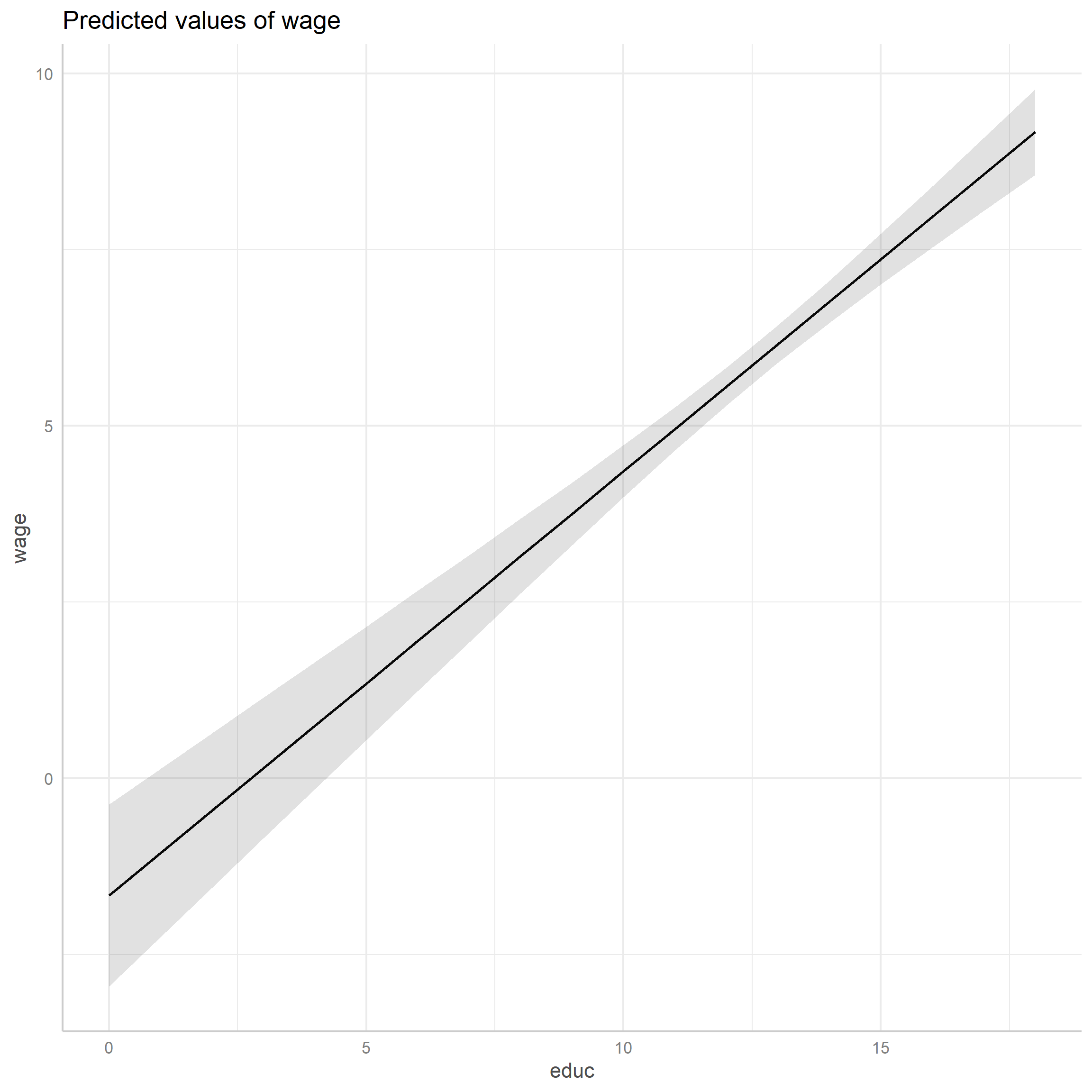
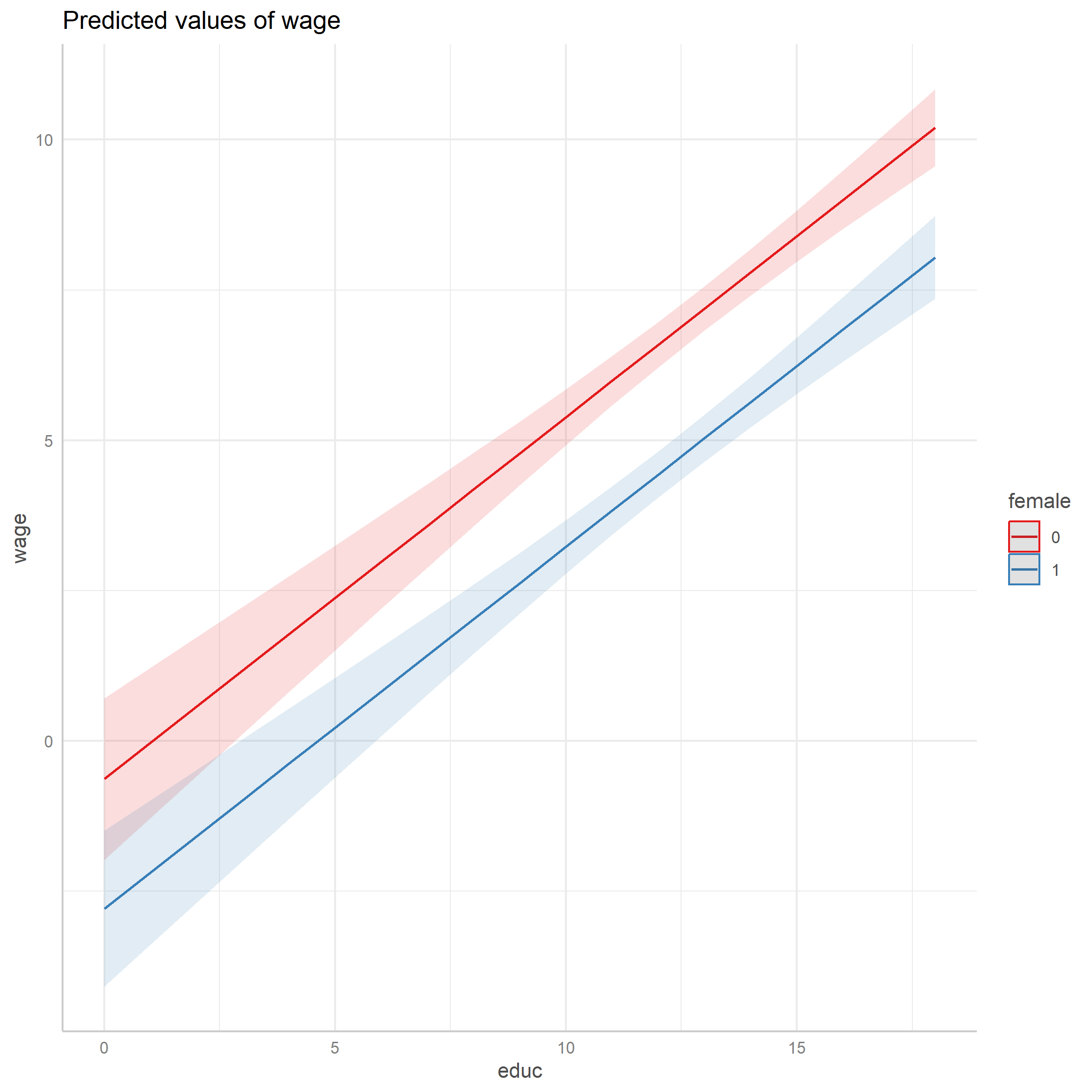

Is model 1 a good predictor of wage based on education?
Is the effect of education causal?
| Model 1 | |
|---|---|
| (Intercept) | -1.715 (0.762)* |
| educ | 0.602 (0.051)*** |
| exper | 0.064 (0.010)*** |
| black | -0.084 (0.444) |
| female | -2.156 (0.271)*** |
| Num.Obs. | 526 |
| R2 Adj. | 0.304 |
| F | 58.341 |
Elasticity is a unit-less measure of change in one variable as a result of a change in the other.
Elasticity of \(y\) with response to \(x\) (\(x\) elasticity of \(y\)):
\[ \epsilon = \frac{\partial y / y}{\partial x / x} = \frac{\partial y}{\partial x} \frac{x}{y} \]
\[ \epsilon = \frac{ \frac{y_2 - y_1}{y_1} }{ \frac{x_2 - x_1}{x_1}} \]
\[ \text{wage} = \beta_0 + \beta_1 \text{educ} + \beta_2 \text{exper} + \beta_3 \text{black} + e \]
Let us compute elasticity of \(\text{wage}\) in response to \(\text{educ}\):
\[ \epsilon_{\text{wage},\text{educ}} = \frac{\partial y}{\partial x} \frac{x}{y}, \]
where: \(\beta_1 = \frac{\partial y}{\partial x}\)
Therefore, elasticity of wage depends on on the value of \(x\) and \(y\).
When elasticity depends on a valued of another variable, we evaluate it at mean (or other quantiles) values of these variables.
| wage | educ | |
|---|---|---|
| mean | 5.90 | 12.56 |
| q2 | 3.33 | 12.00 |
| median | 4.65 | 12.00 |
| q4 | 6.88 | 14.00 |
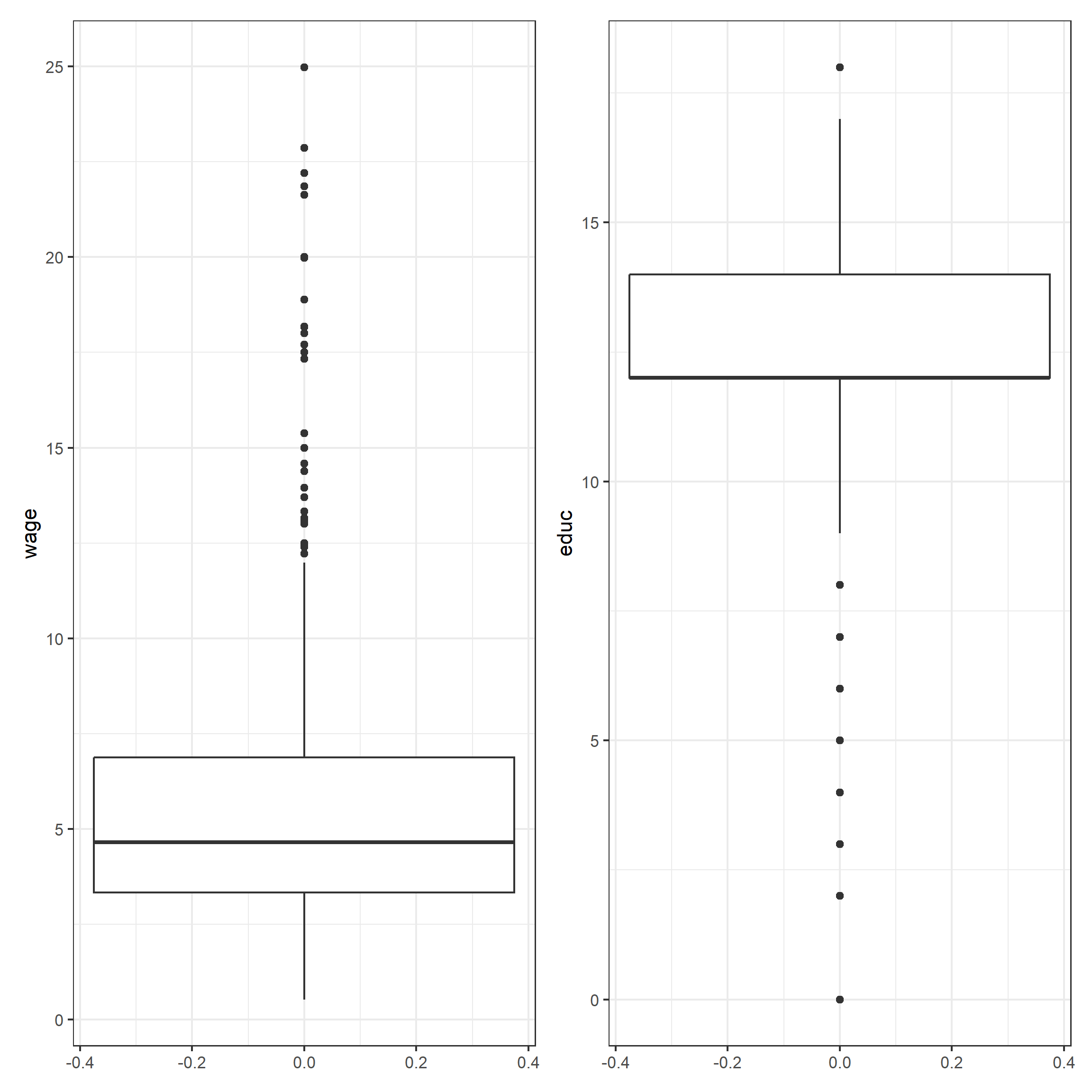

Elasticity at mean:
Elasticity at 2nd, 3rd and 4th quartiles:
Go to the page 2 to refresh motivation for regression assumptions
OLS results with consistent (unbiased) and efficient estimates of population parameters when sample size is finite (\(n \rightarrow \infty\))
\(\hat \beta \rightarrow \beta\)
\(Var(\hat \beta) \rightarrow 0\)
When the sample size is finite and all Gauss-Markov assumptions are satisfied:
\(\hat \beta\) - estimates vary from sample to sample, but
\(Var(\hat \beta)\) is distributed according to the t - distribution.
Variances of two estimates \(Var(\hat \beta_1)\) and \(Var(\hat \beta_2)\) are distributed according to the F - distribution.
When GM assumptions are not satisfied:
t and F distributions are no longer relevant and we cannot perform conduct inference.the expected value of a dependent variable is a straight-line function of the independent variable
If linearity is violated:
estimates are biased
inappropriate representation of the dependent variable
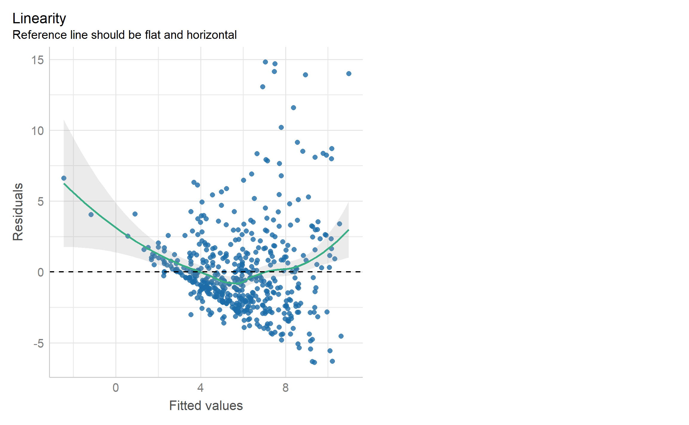
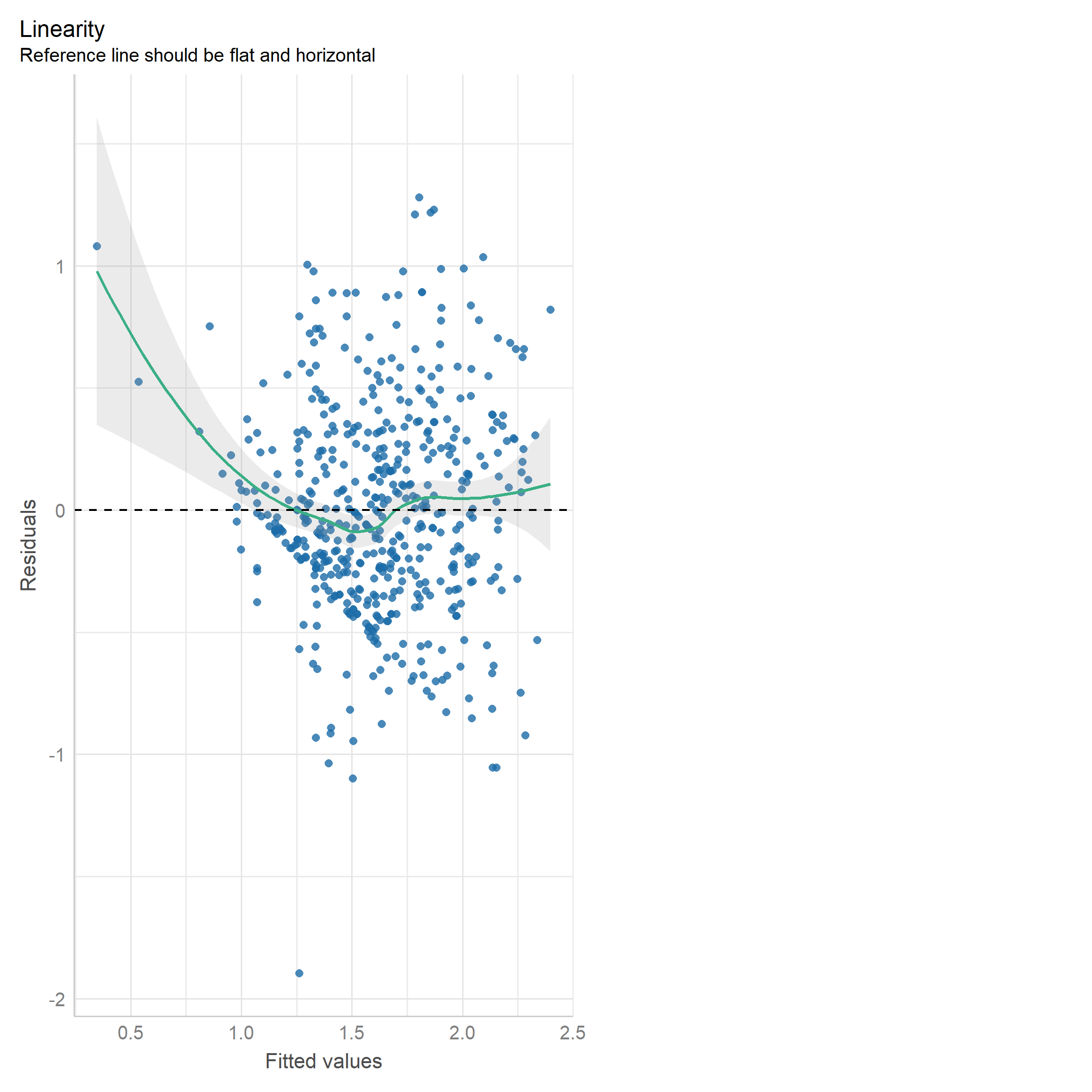
How to detect a non-linearity?
no accepted statistical tests, but
the visual inspection
Typical plots:
Scatter plots of dependent and independent variables;
observed versus predicted/fitted values;
residuals versus predicted/fitted values;
(non) linear transformation to the dependent and/or independent variables;
find a different independent variable;
propose a different functional form;
Interaction term: \(y = \beta_0 + \beta_1 x_1 \cdot x_2 + \beta_2 x_3 + e\)
Natural logarithm: \(\log y = \beta_0 + \beta_2 \log x_1 + \beta_2 x_2 + \beta_3 \log x_3 + e\)
Power transformation and polynomial: \(y = \beta_0 + \beta_2 x_1 ^ 2 + \beta_2 x_2 ^ 3 + \beta_3 \sqrt x_3 + e\)
Box-Cox transformation.
Tailor expansion (Cobb-Douglas, Trans-log).
Reciprocal: \(\log y = \beta_0 + \beta_2 \frac{1}{x_1} + \beta_2 x_2 + \beta_3 \log x_3 + e\)
Standardized variables \(\frac{y - \bar y}{S_y} = \beta_0 + \beta_1 \frac{x_1 - \bar x_1}{S_{x_1}} + \beta_2 \frac{x_2 - \bar x_2}{S_{x_2}} + e\)
| Model | Dep. var. | Indep. var. | Equation | Slope | Interpretation | Elasticity |
|---|---|---|---|---|---|---|
| \(\frac{\partial y}{\partial x}\) | \(\frac{\partial y}{\partial x} \cdot \frac{x}{y}\) | |||||
| Level - level | \(y\) | \(y\) | \(y=\beta_0 + \beta_1 x\) | \(\beta_1\) | \(\Delta y = \beta_1 \Delta x\) | \(\beta_1 \frac{x}{y}\) |
| Level - log | \(y\) | \(\log x\) | \(\log y=\beta_0 + \beta_1 x\) | \(\beta_1 y\) | \(\Delta y = (\beta_1/100)\% \Delta x\) | \(\beta_1 x\) |
| Log - level | \(\log y\) | \(x\) | \(y=\beta_0 + \beta_1 \log x\) | \(\beta_1 \frac{1}{x}\) | \(\% \Delta y = 100 \beta_1 \Delta x\) | \(\beta_1 \frac{1}{y}\) |
| Log - log | \(\log y\) | \(\log x\) | \(\log y=\beta_0 + \beta_1 \log x\) | \(\beta_1 \frac{y}{x}\) | \(\% \Delta y = \% \beta_1 \Delta x\) | \(\beta_1\) |
\(\log(0) = - \infty\);
what is the \(\log(x)\), when \(x < 0\)?
| Model | Dep. var. | Indep. var. | Equation | Slope | Interpretation | Elasticity |
|---|---|---|---|---|---|---|
| \(\frac{\partial y}{\partial x}\) | \(\frac{\partial y}{\partial x} \cdot \frac{x}{y}\) | |||||
| Standardized variables | \(y^* = \frac{y - \bar y}{S_y}\) | \(x^* = \frac{x - \bar x}{S_x}\) | \(y^*=\beta_0 + \beta_1 x^*\) | \(\frac{\partial y^*}{\partial x^*}\) | \(\text{SD} \Delta y = \text{SD} \beta_1 \Delta x\) | DIY |
Key limitations:
| Model | Dep. var. | Indep. var. | Equation | Slope | Elasticity |
|---|---|---|---|---|---|
| \(\frac{\partial y}{\partial x}\) | \(\frac{\partial y}{\partial x} \cdot \frac{x}{y}\) | ||||
| Reciprocal | \(y\) | \(\frac{1}{x}\) | \(y=\beta_0 + \beta_1 \frac{1}{x}\) | \(-\beta_1 \frac{1}{x^2}\) | \(-\beta_1 \frac{1}{xy}\) |
Interpretation:
See Gujarati (2004) Chapter 6.7 for more details on interpreting the reciprocal relationship.
Call:
lm(formula = log(wage) ~ educ + exper + black + female, data = wage_dta)
Coefficients:
(Intercept) educ exper black female
0.483188 0.091192 0.009411 -0.009889 -0.343712
Call:
lm(formula = log(wage) ~ educ + exper + black + female, data = wage_dta)
Residuals:
Min 1Q Median 3Q Max
-1.89689 -0.26333 -0.03394 0.26654 1.28131
Coefficients:
Estimate Std. Error t value Pr(>|t|)
(Intercept) 0.483188 0.106141 4.552 6.61e-06 ***
educ 0.091192 0.007156 12.743 < 2e-16 ***
exper 0.009411 0.001451 6.487 2.04e-10 ***
black -0.009889 0.061913 -0.160 0.873
female -0.343712 0.037709 -9.115 < 2e-16 ***
---
Signif. codes: 0 '***' 0.001 '**' 0.01 '*' 0.05 '.' 0.1 ' ' 1
Residual standard error: 0.4293 on 521 degrees of freedom
Multiple R-squared: 0.3526, Adjusted R-squared: 0.3476
F-statistic: 70.93 on 4 and 521 DF, p-value: < 2.2e-16


| Model 1 (level-level) | Model 2 (log(wage)-level) | |
|---|---|---|
| (Intercept) | -1.715 (0.762)* | 0.483 (0.106)*** |
| educ | 0.602 (0.051)*** | 0.091 (0.007)*** |
| exper | 0.064 (0.010)*** | 0.009 (0.001)*** |
| black | -0.084 (0.444) | -0.010 (0.062) |
| female | -2.156 (0.271)*** | -0.344 (0.038)*** |
| Num.Obs. | 526 | 526 |
| R2 Adj. | 0.304 | 0.348 |
| F | 58.341 | 70.934 |
No collinearity means
For example:
biased estimates of the collinear variables
over-significant results;
Scatter plot; Correlation matrix;
Model specification;
Step-wise regression approach;
Variance Inflation Factor;
Re specify the model;
Choose different regressors;
See also:
Overview: “Assumption AMLR.3 No Perfect Collinearity” in (Wooldridge, 2020) ;
Examples of causes in Chapter 9.5 (Wooldridge, 2020) ;
Chapter 9.4-9.5 in (Weisberg, 2005);
We want to build a naive regression, where the wage is a function of sex (female and male):
\(\text{wage} = \beta_0 + \beta_1 \cdot \text{female} + \beta_2 \cdot \text{male}\)
The data is fictional:
Rows: 14
Columns: 3
$ female <int> 1, 1, 0, 0, 1, 1, 1, 0, 0, 1, 1, 0, 1, 1
$ male <int> 0, 0, 1, 1, 0, 0, 0, 1, 1, 0, 0, 1, 0, 0
$ wage <dbl> 10.847522, 7.167989, 4.941890, 7.477957, 9.391538, 8.087289, 9.…
| Model 1 | Model 2 | Model 3 | Model 4 | Model 5 | |
|---|---|---|---|---|---|
| (Intercept) | 8.747*** (0.468) | 6.094*** (0.628) | 6.094*** (0.628) | ||
| male | -2.652** (0.784) | 6.094*** (0.628) | 6.094*** (0.628) | ||
| female | 2.652** (0.784) | 2.652** (0.784) | 8.747*** (0.468) | 8.747*** (0.468) | |
| Num.Obs. | 14 | 14 | 14 | 14 | 14 |
| R2 | 0.488 | 0.488 | 0.488 | 0.974 | 0.974 |
| R2 Adj. | 0.446 | 0.446 | 0.446 | 0.969 | 0.969 |
Note: ^^ Model 1: wage ~ male
Model 2: wage ~ female
Model 3: wage ~ female + male
Model 4: wage ~ 0 + female + male
Model 5: wage ~ 0 + male + female
| Model 1 | Model 2 | Model 3 | |
|---|---|---|---|
| (Intercept) | 8.747*** (0.468) | 6.094*** (0.628) | 6.094*** (0.628) |
| male | -2.652** (0.784) | ||
| female | 2.652** (0.784) | 2.652** (0.784) | |
| Num.Obs. | 14 | 14 | 14 |
| R2 | 0.488 | 0.488 | 0.488 |
| R2 Adj. | 0.446 | 0.446 | 0.446 |
Note: ^^ Model 1: wage ~ male
Model 2: wage ~ female
Model 3: wage ~ female + male
| Model 1 | Model 2 | Model 3 | Model 4 | |
|---|---|---|---|---|
| (Intercept) | 8.747*** (0.468) | 6.094*** (0.628) | 6.094*** (0.628) | |
| male | -2.652** (0.784) | 6.094*** (0.628) | ||
| female | 2.652** (0.784) | 2.652** (0.784) | 8.747*** (0.468) | |
| Num.Obs. | 14 | 14 | 14 | 14 |
| R2 | 0.488 | 0.488 | 0.488 | 0.974 |
| R2 Adj. | 0.446 | 0.446 | 0.446 | 0.969 |
Note: ^^ Model 1: wage ~ male
Model 2: wage ~ female
Model 3: wage ~ female + male
Model 4: wage ~ 0 + female + male
Watch these videos on youtube and read
Video 1: Ceteris Paribus: Public vs. Private University or this link: https://youtu.be/iPBV3BlV7jk
Re watch video 2: Selection Bias or this link: https://youtu.be/6YrIDhaUQOE
Read:
(Angrist & Pischke, 2014, Chapter 2; optional Angrist & Pischke, 2009, Chapter 3)
Do:
Follow pre-recorded videos in the order below. Please note that slides below supplement some of those practical works.
\[ \pmb{y} = \pmb{x}\beta+\pmb{e} \]
where
\[ \pmb{e} = \pmb{y} - \pmb{x}\hat \beta \]
Dependent variable:
\[ \pmb{y} = \begin{bmatrix} y_1 \\ y_2 \\ \vdots \\ y_k \end{bmatrix} \]
Independent variables:
\[ \pmb{x} = \begin{bmatrix} 1 & x_{11} & x_{12} & \dots & x_{1n} \\ 1 & x_{21} & x_{22} & \dots & x_{2n} \\ \vdots & \vdots & \vdots & \ddots & \vdots \\ 1 & x_{k1} & x_{k2} & \dots& x_{kn} \\ \end{bmatrix} \]
\[ \hat \beta = \begin{bmatrix} \hat \beta_0 & \hat \beta_1 & \hat \beta_2 & \cdots & \hat \beta_n \end{bmatrix} \]
\[ \pmb{y} = \pmb{x}\hat\beta \]
\[ \pmb{x}^{T} \pmb{y} = \pmb{x}^{T} \pmb{x_i}\hat\beta \]
\[ \frac{1}{ \pmb{x}^{T} \pmb{x_i}} \pmb{x}^{T} \pmb{y} = \frac{1}{ \pmb{x}^{T} \pmb{x_i}}\pmb{x}^{T} \pmb{x_i}\hat\beta \]
\[ (\pmb{x}^{T} \pmb{x_i}) ^ {-1} \pmb{x}^{T} \pmb{y} = \hat\beta \]
where:
\(\pmb{x}^{T}\) is the transposed matrix \(\pmb{x}\)
\((\cdot) ^ {-1}\) is the inverse of a matrix
\[ \pmb{\hat y} = \pmb{x} \hat\beta = \begin{bmatrix} 1 & x_{11} & x_{12} & \dots & x_{1n} \\ 1 & x_{21} & x_{22} & \dots & x_{2n} \\ \vdots & \vdots & \vdots & \ddots & \vdots \\ 1 & x_{k1} & x_{k2} & \dots& x_{kn} \\ \end{bmatrix} \begin{bmatrix} \hat \beta_0 \\ \hat \beta_1 \\ \hat \beta_2 \\ \vdots \\ \hat \beta_n \end{bmatrix} = \]
\[ \begin{bmatrix} \beta_0 + \beta_1 x_{11} + \beta_2 x_{12} + \dots + \beta_n x_{1n} \\ \beta_0 + \beta_1 x_{21} + \beta_2 x_{22} + \dots + \beta_n x_{2n} \\ \vdots \\ \beta_0 + \beta_1 x_{k1} + \beta_2 x_{k2} + \dots + \beta_n x_{kn} \\ \end{bmatrix} = \begin{bmatrix} \hat y_1 \\ \hat y_2 \\ \vdots \\ \hat y_k \end{bmatrix} \]
\[ \pmb{\hat e} = \pmb{y} - \pmb{\hat y} = \begin{bmatrix} y_1 - \hat y_1 \\ y_2 - \hat y_2 \\ \vdots \\ y_k - \hat y_k \end{bmatrix} = \begin{bmatrix} \hat e_1 \\ \hat e_2 \\ \vdots \\ \hat e_k \end{bmatrix} \]
Measure of variance in the estimated parameters \(\beta\). Computed based on the Variance Covariance matrix
\[ Var(\hat \beta) = (\pmb{x}^T \pmb{x})^{-1} \hat \sigma_e \]
where \(\hat \sigma_e\) is the estimate of the variance in error terms:
\[ \hat \sigma_e = \frac{\pmb{\hat e}^T\pmb{\hat e}}{n-r} \]
\(n\) - number of observations and \(r\) number of regressors including intercept.
Standard Errors:
\[ \text{SE} = \sqrt{\text{diag}(Var(\hat \beta) )} \]
SE are needed for the inference!
To conclude about the population based on the sample regression results.
Get comfortable with the terminology:
Control variables for creating Ceteris Paribus
Selection Bias in Regression:
OVB;
Long and Short models;
Regression components and how do one produce them:
Why assumptions are important?
Linearity and how to detect it?
What is perfect collinearity?