Week 06. Recap. Simple Linear Regression. Multiple Regression. Bias. Regression assumptions. Linearity.

Part 1: Statistics and Econometrics. MK68-2024/25

Justus Liebig University Giessen

Institute of Agricultural Policy and Market Research

Example of an exam assignment

The slides below show you what you can expect on an exam based on the material of the past weeks.

Please note that:

  • these examples exaggerated the complexity of the exam.

Definition question

Answer two questions from the list below:

  • What measures of central tendency are most commonly applied in social sciences?

  • What are extreme observations or outliers?

  • What effect do outliers/extreme observations have on the mean/median, standard deviation/IQR?

  • Is the median one of the quantiles or is it a measure of central tendency?

  • What is the Hypothesis Testing?

Problem introduction

An RCT experiment was designed to understand the effect of technology (“Minimal” vs “Optimal”) on rice yields. It included:

  1. Randomly selecting 60 farms and offering them two equivalent rice varieties to plant.

    • each farmer picked one variety randomly.
  2. Training half of them in applying Optimal technology (treatment), and

  3. Keeping half of the farmers with the same minimal technology (control).

During the production season, researchers recorded for each farm:

  • Technology, rice variety, rice yield, and fertilizer use.

  • The research objective was to measure the effect of technology on rice yield.

Answer the questions on the following slides based on this example.

Descriptive analysis (1)

Continuous variables

Unique Missing Pct. Mean SD Min Median Max
yield 60 0 5.4 1.1 3.1 5.4 7.9
nitrogen 52 0 77.3 49.6 0.0 79.0 148.6
potassium 60 0 33.1 15.1 1.7 34.3 61.4
phosphorus 60 0 37.6 21.6 0.8 38.8 74.7

Categorical variables

N %
tech Minimum (control) 30 50.0
Optimum (treatment) 30 50.0
variety V1 30 50.0
V2 30 50.0

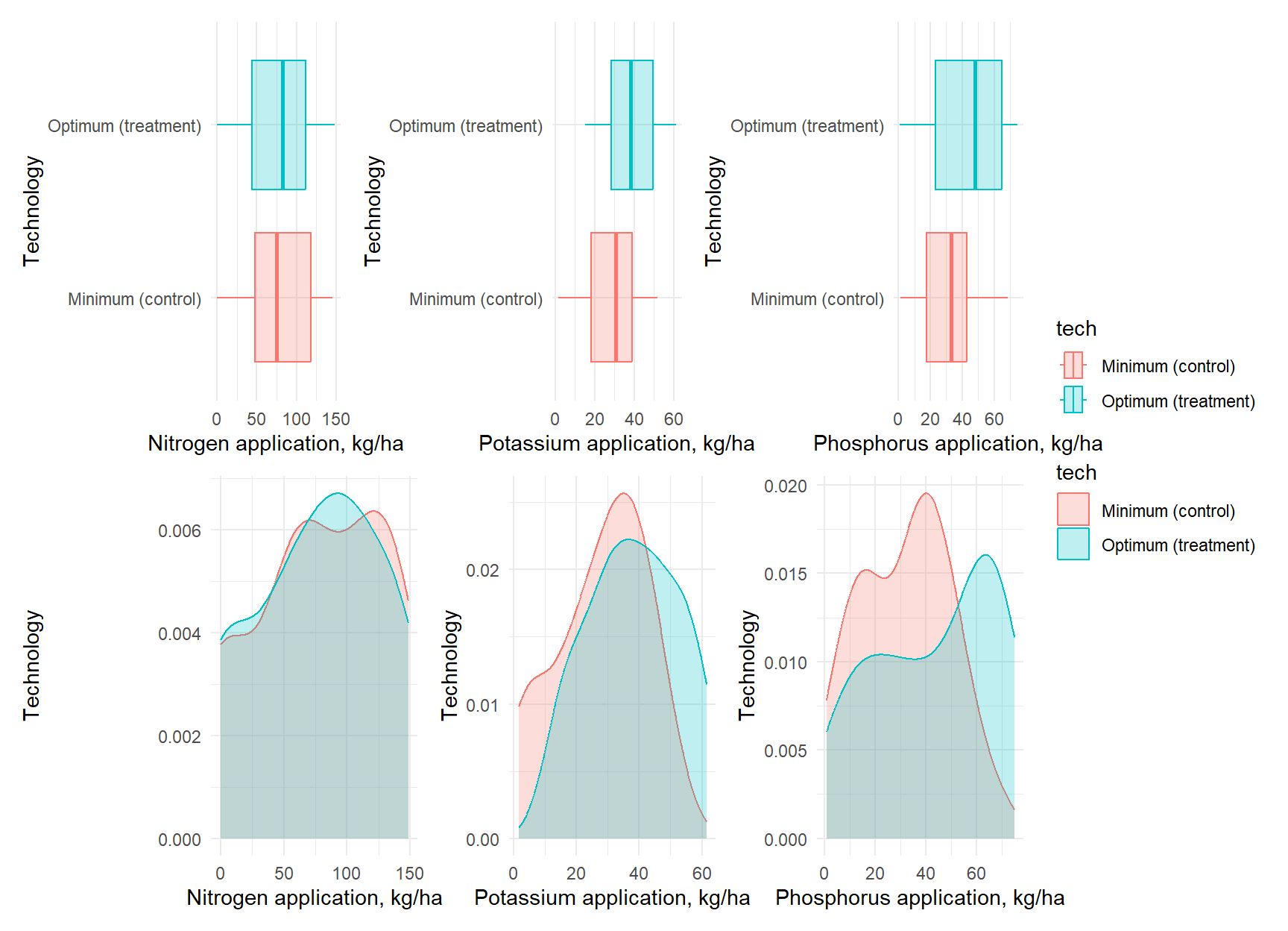
Checks and Balances (1)

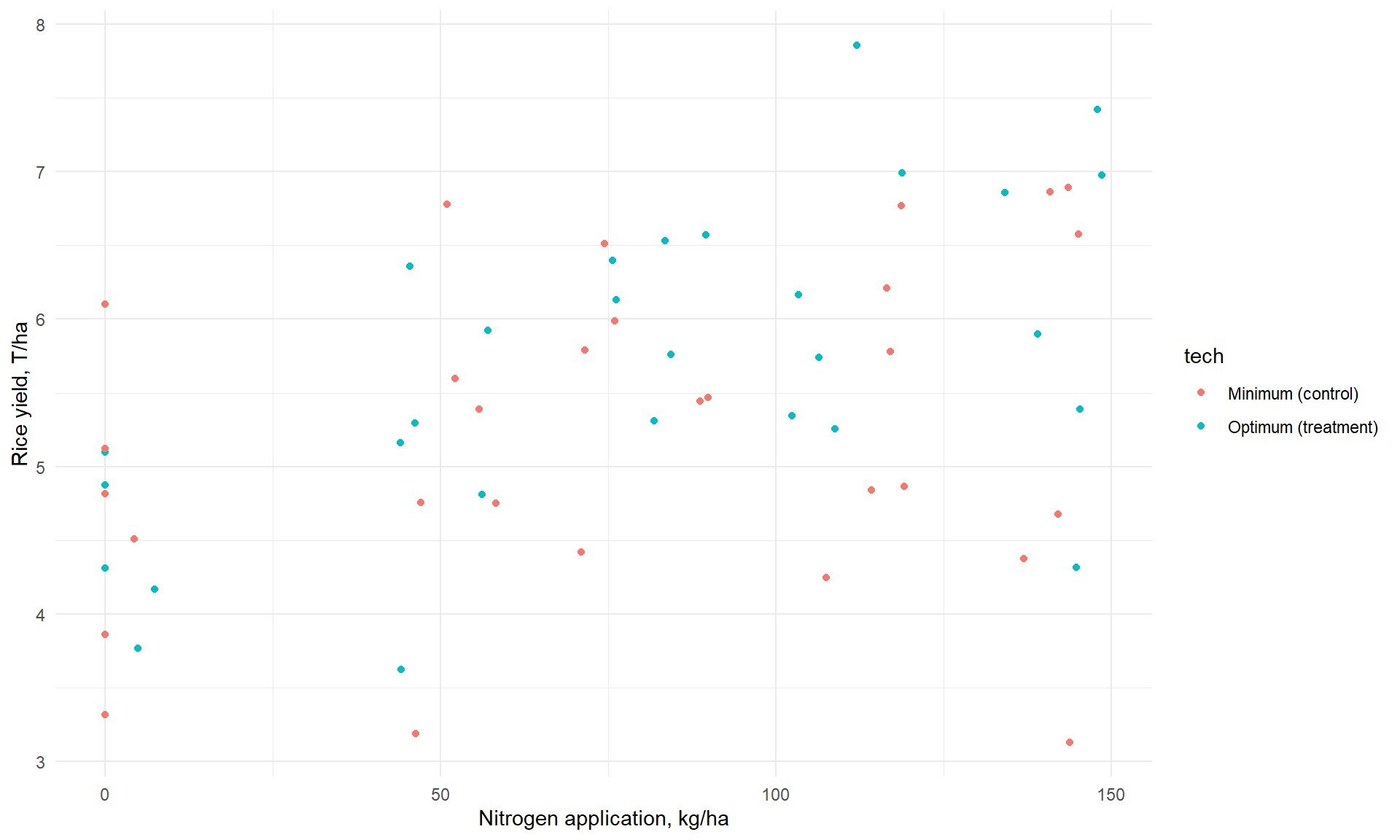
  • What differences do you observe between technologies in terms of the fertilizers used?

  • What can we conclude about the quality of random assignment based on this plot?

Checks and Balances (2)

Minimum (control) (N=30)
Optimum (treatment) (N=30)
Mean Std. Dev. Mean Std. Dev.
nitrogen 77.7 50.4 76.9 49.7
potassium 28.0 14.4 38.2 14.2
phosphorus 31.7 17.9 43.4 23.7

Significance levels are: ‘+’=.1, ‘*’=.05, ‘**’=.01, ‘***’=0.001

  • Perform hypothesis testing about the difference in mean fertilizer application between the two technologies.

  • What can we conclude about the quality of random assignment based on this table?

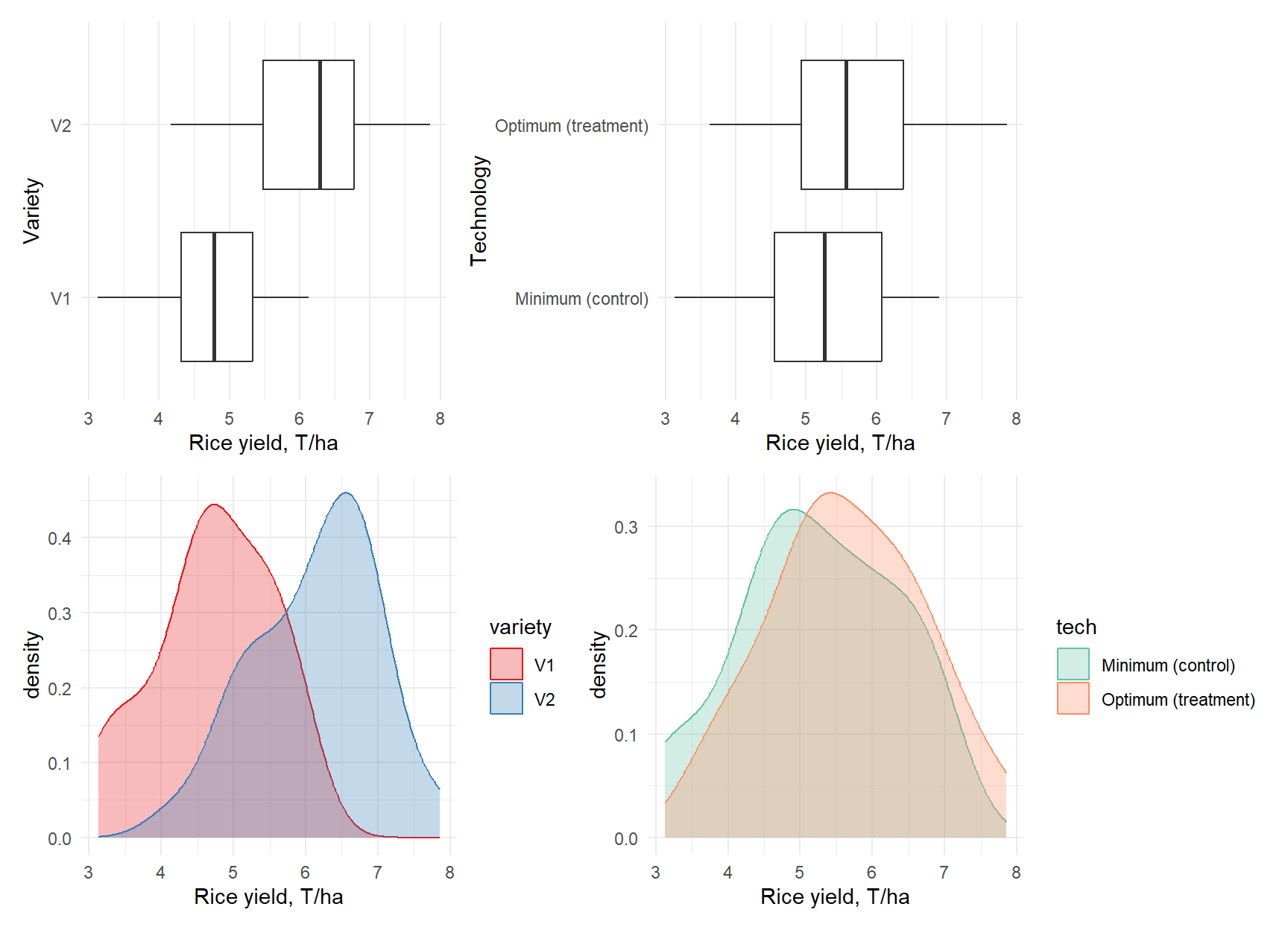
Effect of technology on yields

  • Our key objective is to quantify the effect of technology on yields.

  • What differences do you observe between technologies in terms of rice yields?

  • Can we conclude about the causal effect of technologies based on this plot?

HT: effect of technology on yields

Minimum (control) (N=30)
Optimum (treatment) (N=30)
Mean Std. Dev. Mean Std. Dev.
yield 5.2 1.1 5.6 1.1

Significance levels are: ‘+’=.1, ‘*’=.05, ‘**’=.01, ‘***’=0.001

  • Why do we need this HT?

  • Formulate H0 and H1.

  • Conclude about the effect of technology on yields.

  • What statistics did you use?

  • What is the highest level of significance for your results?

Conclude about the effect of technology on yields

  • Does the optimal technology have any causal effect on yields?

  • How large is this effect?

  • Does the RCT performed here ensures the ceteris paribus?

  • What else can influence the effect of technology on yield?

  • How can we control for it?

Differences in yields between varieties
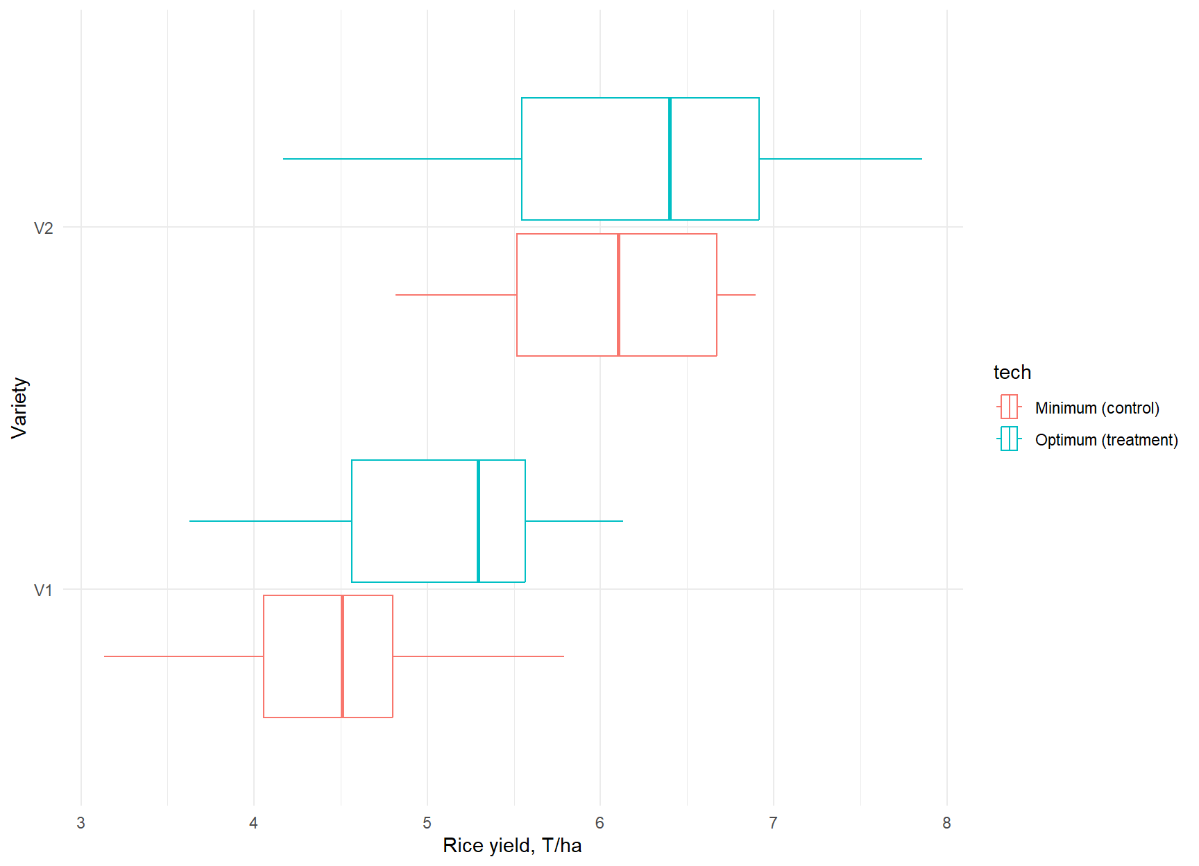
  • What does this plot show?

  • Considering previous results, can we conclude about the quality of random assignment now?

  • Is there a causal effect of variety on yields, which effect is this?

HT: effect of variety on yields

V1 (N=30)
V2 (N=30)
Mean Std. Dev. Mean Std. Dev.
yield 4.7 0.8 6.1 0.9

Significance levels are: ‘+’=.1, ‘*’=.05, ‘**’=.01, ‘***’=0.001

  • Formulate H0 and H1.

  • Conclude about the yield difference between varieties.

  • Based on our sample, can we conclude that variety has a causal effect on yields?

  • Does our sample ensure the ceteris paribus? How does our sample ensure it?

Conclude again

  • Does the random assignment of technology ensure the ceteris paribus here?

  • What are the most relevant other factors that may influence the ceteris paribus in our sample?

  • Given that what can we conclude about the causal effect of technology on yields?

  • After today’s lecture you should be able to answer the following:

    • Can we “control” the effects of the other factors?

    • What econometric method can we use to re-establish the ceteris paribus?

    • How (can we at all) measure the effects of other factors such as fertilizer application on the yields?

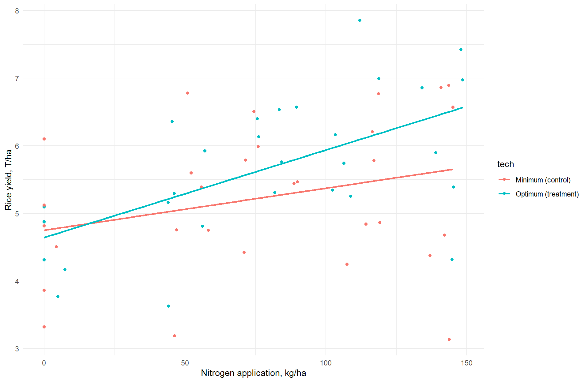
How to measure the effect of nitrogen fertilizer on yield?
Framework for interpreting any statistical test

For your reference and information.

The keywords/concepts below are meant to improve the clarity of communication when performing the hypothesis testing. Please use it! They will help make your results understandable for the reader.

  1. Test name and what it is about (t-test about means comparison between two groups).

  2. \(H_0\) and \(H_1\).

  3. Estimated parameters (means, coefficients, differences, standard error), \(df\) / n observations.

  4. Level of significance of the HT. (\(\alpha = 0.05\) or 5% level of significance)

  5. Rejection rule: \(\text{p-value} < \alpha\) or \(|t| < c_{df, \, 1 - \alpha /2}\) (statistics vs critical value) or \(1 - \alpha\) confidence intervals (95% CI).

  6. Conclusions: reject/fail to reject;

  7. Implications

    • what do these conclusions imply for your analysis?

    • (for example. … reject \(H_0\). Thus, the mean “outcome” in the treatment group XX is higher than that in the control group, suggesting about the great success of our intervention …).

(Very) Simple Linear Regression

two-variables linear or bi-variate linear regression model.

Explains how \(y\) the Dependent variable varies with changes in \(x\) the independent variable.

SLR on population and sample

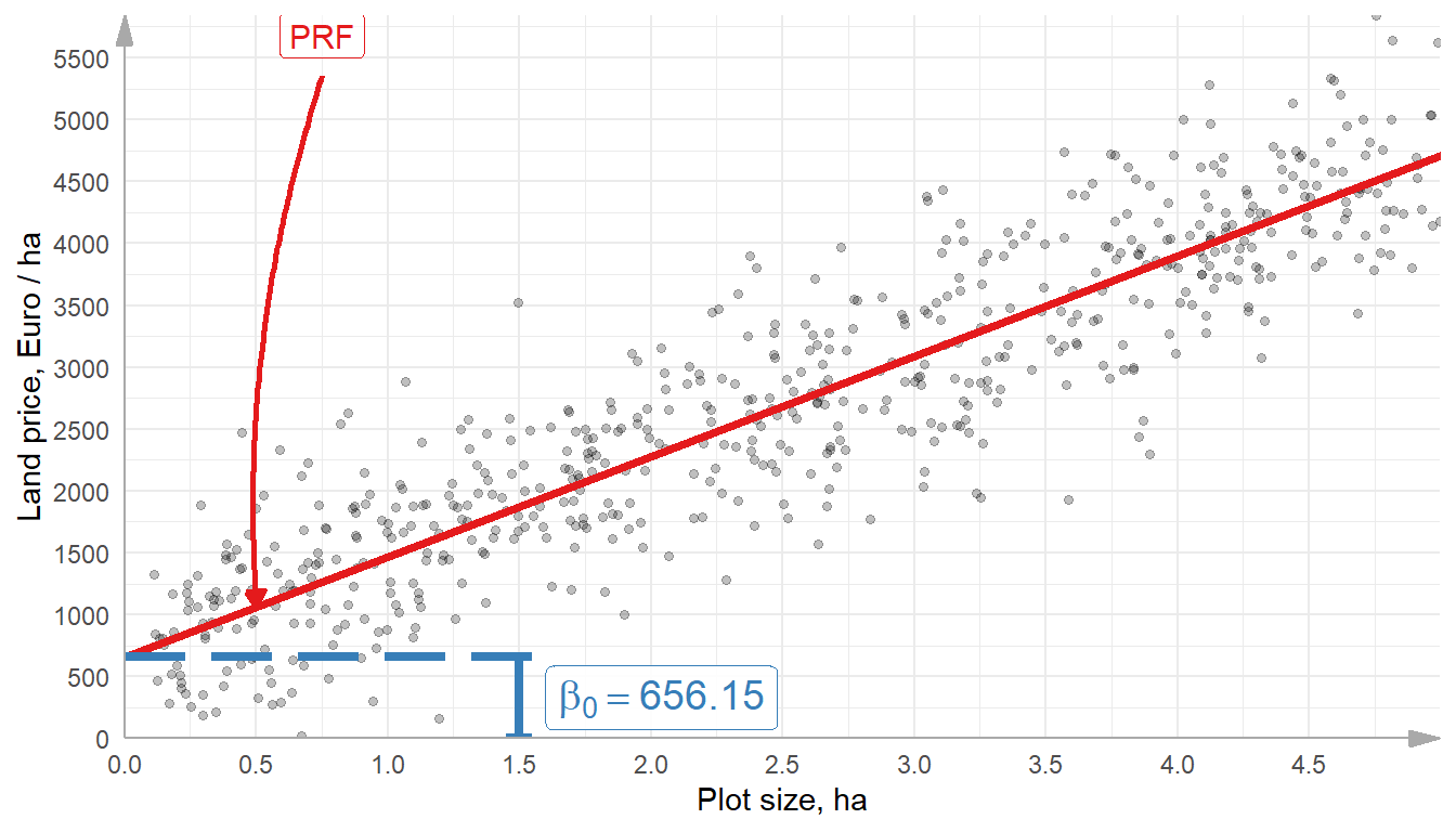
Population regression (PRF)

Always unknown

\[y = {\beta}_{0} + {\beta}_{1}x + u\]

  • \(y\) - dependent variable
  • \(x\) - independent variable
  • \({\beta}_{0}\) - the true value of the intercept (constant term)
  • \({\beta}_{1}\) - the true value of the slope
  • \(u\) - the true value of the error term or disturbance

Estimated regression

What we learn from the sample of size \(n\), where \(i \in {1, 2, \dots, n}\)

\[y_i = \hat{\beta}_{0} + \hat{\beta}_{1} x_i + \hat{u_i}\]

  • \(y_i\) - dependent variable from \(i\) obs. in the sample
  • \(x_i\) - independent variable
  • \(\hat{\beta}_{0}\) - estimated intercept (constant term)
  • \(\hat{\beta}_{1}\) - estimated slope
  • \(\hat{u_i}\) - estimated error term or disturbance

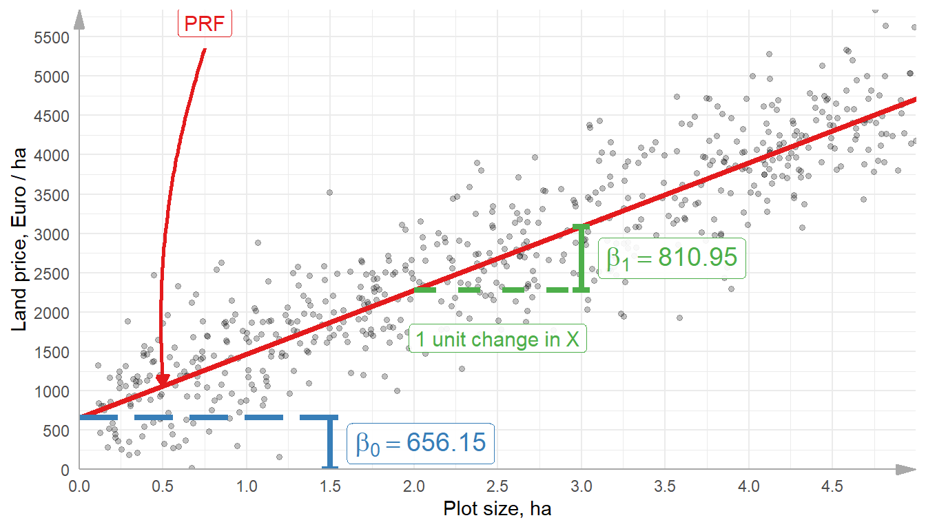
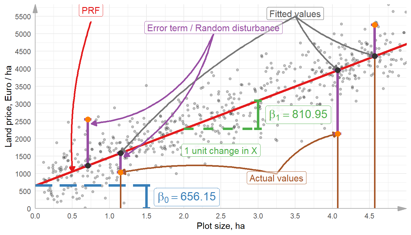
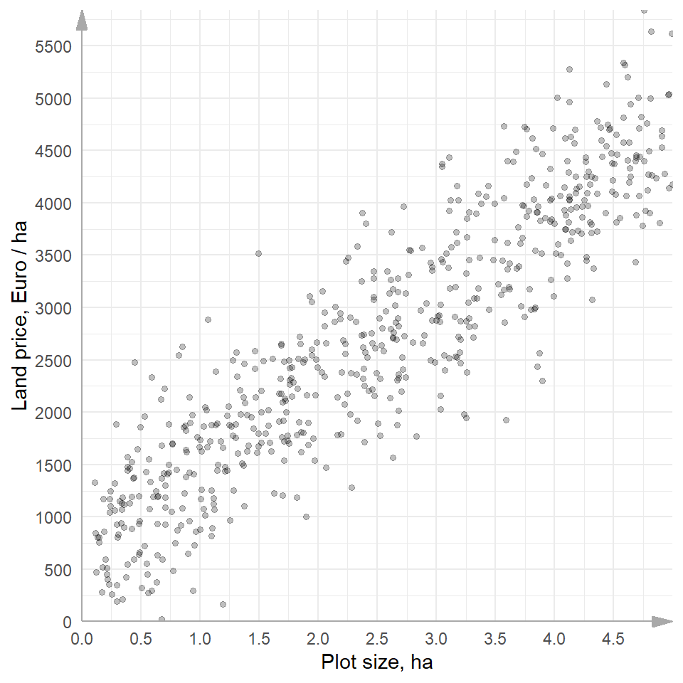
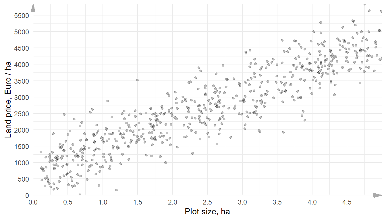
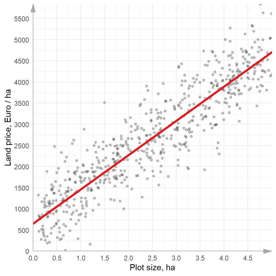
Plot size and farmland prices

We simulate a population of \(2\times 10^{6}\) agricultural fields. Each field has only two characteristics:

  • price of 1 ha of land in in a land plot in Euro
  • size of a land plot in ha

Each field could be different in quality of soil, landscape, accessibility but we assume that the other things are equal.
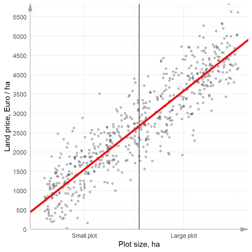
Regression Line
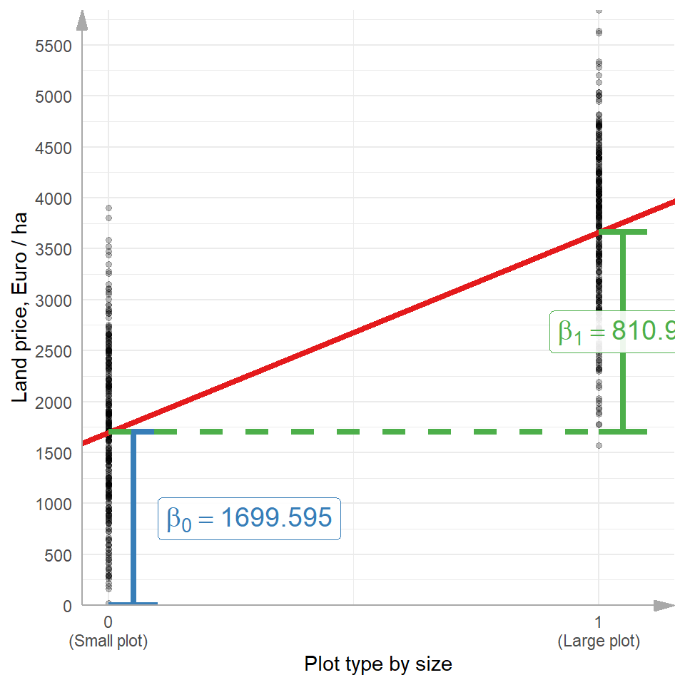
Regression Line (cont.)
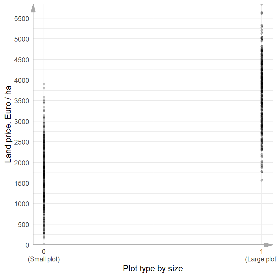
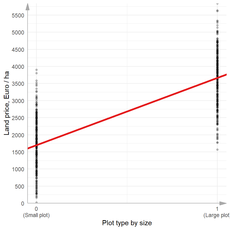
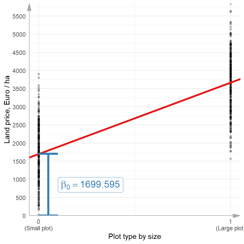
plot_large is a dummy variable also called an “indicator variable”

# A tibble: 600 × 4
    area value plot_size  plot_large
   <dbl> <dbl> <fct>           <dbl>
 1 3.79  3180. Large plot          1
 2 3.01  2920. Large plot          1
 3 1.10  1252. Small plot          0
 4 1.06  1669. Small plot          0
 5 2.23  2656. Small plot          0
 6 4.11  3276. Large plot          1
 7 3.65  4393. Large plot          1
 8 0.705  928. Small plot          0
 9 4.30  4179. Large plot          1
10 1.09  1720. Small plot          0
11 3.77  3869. Large plot          1
12 1.85  2655. Small plot          0
# ℹ 588 more rows
Regression Line (cont.)
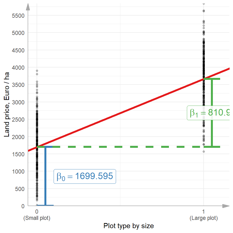
t.test(value ~ plot_size, plot_pop_dta2)
#   Welch Two Sample t-test
# data:  value by plot_size
# t = -29.887, df = 594.75, p-value < 2.2e-16
# alternative hypothesis: true difference in means 
#    between group Small plot and group Large plot 
#    is not equal to 0
# 95 percent confidence interval:
#  -2094.443 -1836.148
# sample estimates:
# mean in group Small plot 
#                 1699.595
# mean in group Large plot 
#                 3664.890 

Regression: Coefficients

Regression parameters / coefficient (\(\hat{\beta}_0\) and \(\hat{\beta}_1\)) are estimated using the Ordinary Least Squares (OLS) method. These are:

The intercept: (\(\hat{\beta}_0\))

  • is the value of \(\hat{y}\), when all regressors (\(x\)) are zero.

The slope: (\(\hat{\beta}_1\))

  • change in the expected value of \(\hat{y}\) (in units of \(y\)), when \(x\) increases by one unit.

Regression: Coefficients interpretation
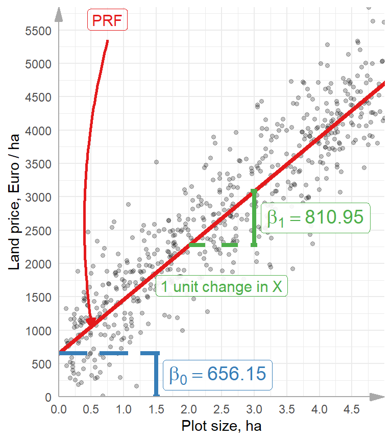
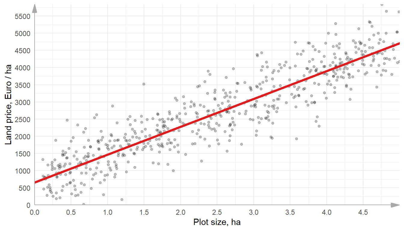
In the example of land price, where \(\hat{\beta_0} = 656.15\) and \(\hat{\beta_1} = 810.95\):

Intercept:

  • On average, starting price of a land plot with near to zero size is 656.15 Euros per ha.

Slope:

  • The expected price of 1 ha of land increases by 810.95 Euros when the plot size increases by 1 HA

Regression: OLS Algorithm
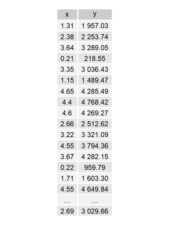
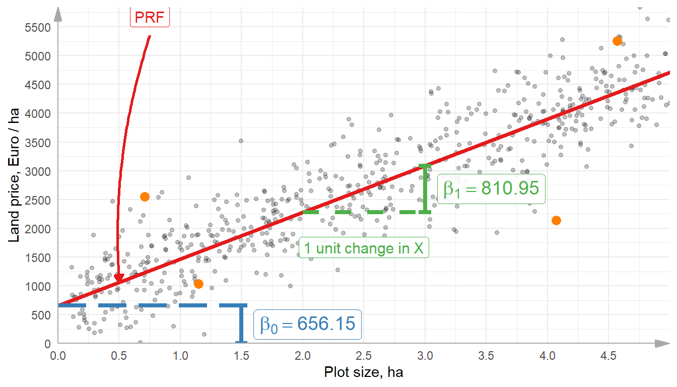
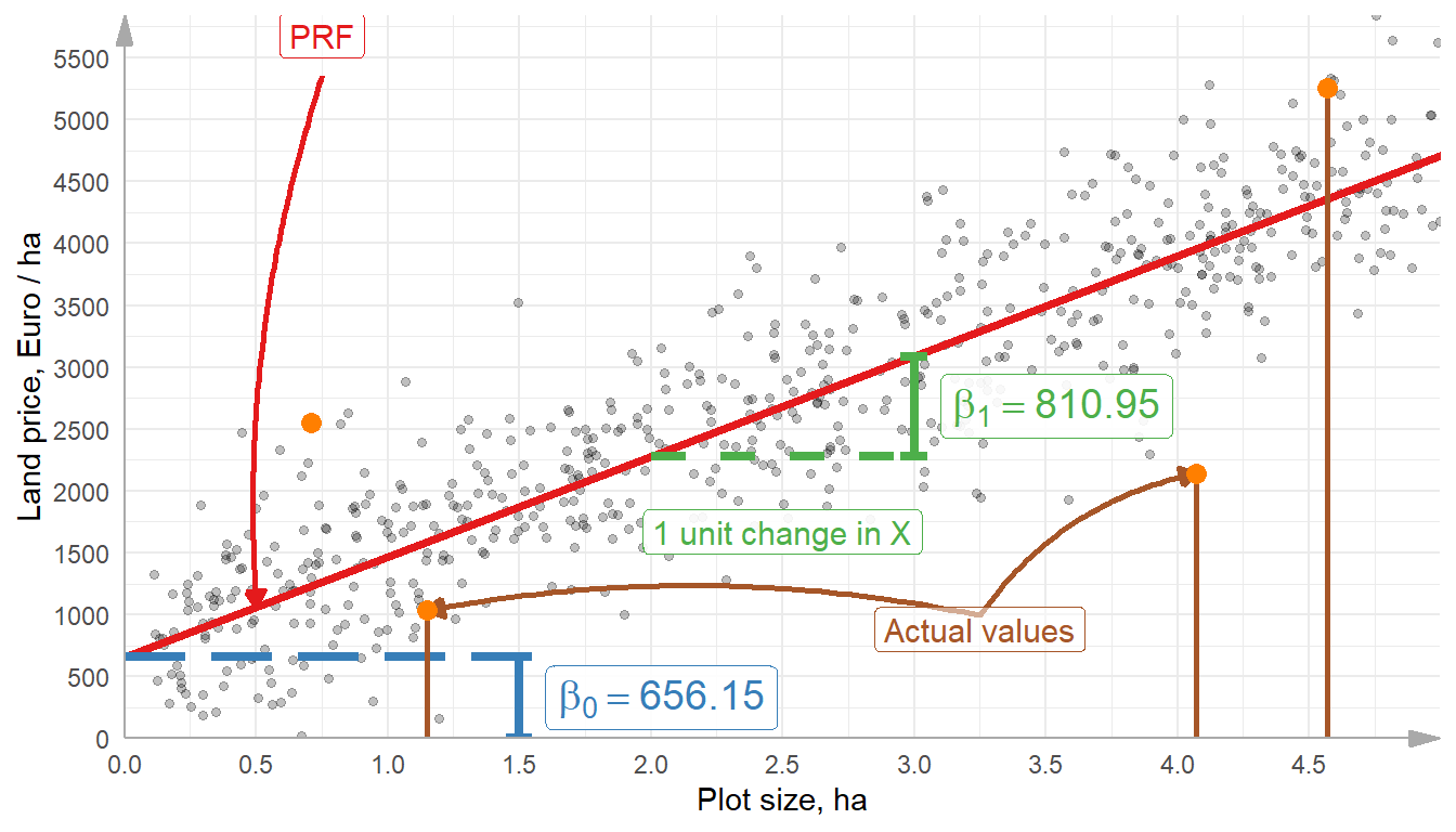
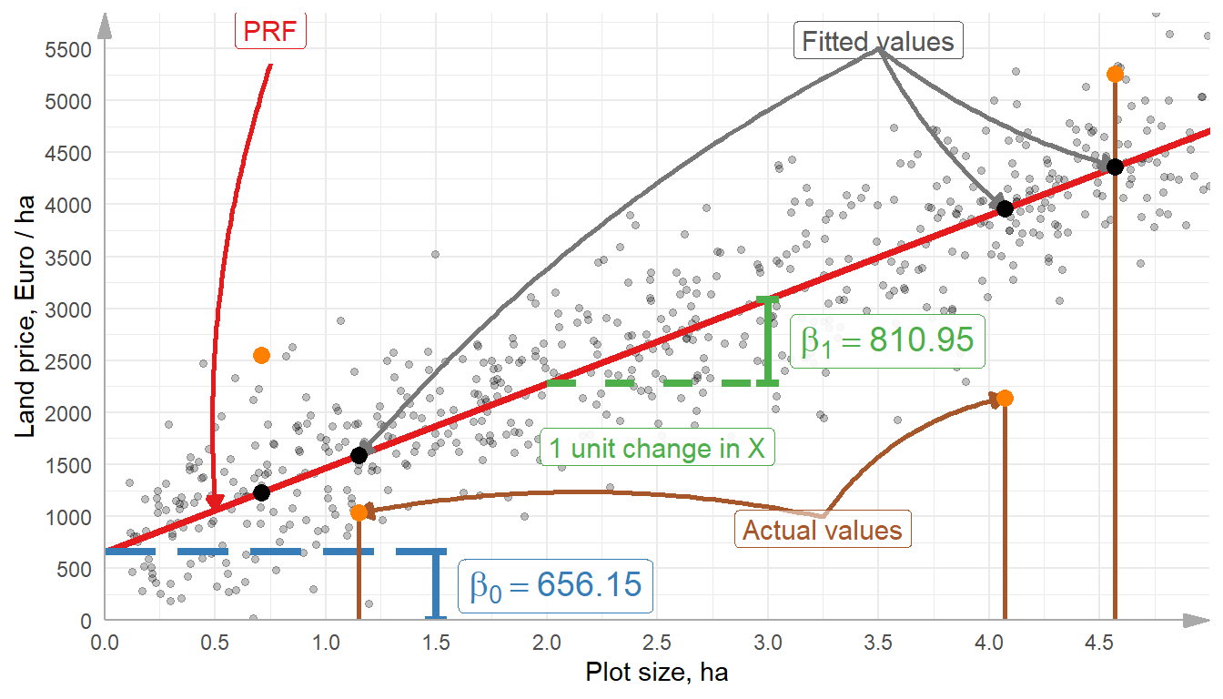
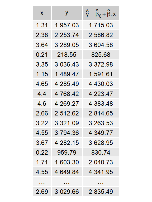
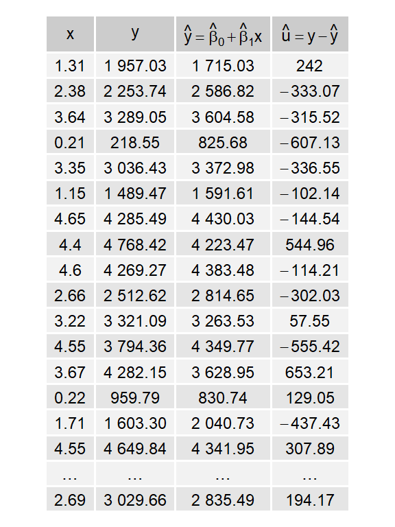
1 Proposes \(\hat{\beta_0}\) and \(\hat{\beta_1}\) so that actual values are: \(y_i = \hat{\beta}_0 + \hat{\beta}_1 \cdot x_i + \hat{u}_i\)

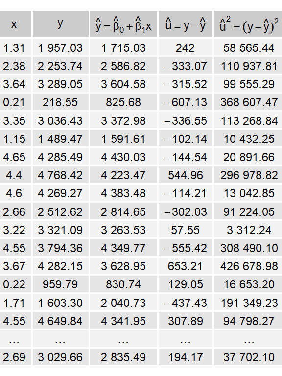
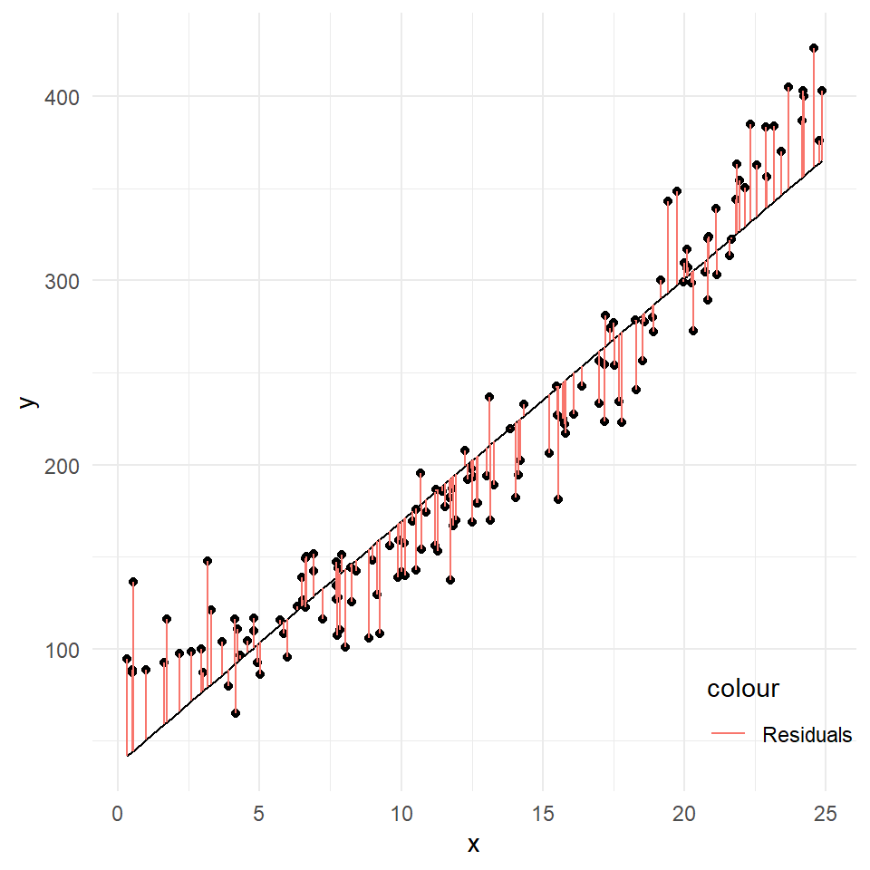
2 Computes fitted values (\(\hat{y}_i = \hat{\beta}_0 + \hat{\beta}_1 \cdot x_i\)) and residuals (\(\hat{u}_i = y_i - \hat{y}_i\)).

3 Computes squared residuals and the sum of it \(\sum \hat{u}^2\)

4 Repeats 1-3 with new estimates of \(\hat{\beta_0}\) and \(\hat{\beta_1}\);

5 Compare new sum of squared residuals \(\sum \hat{u}\) to the previous one.

6 Repeats 4-5 to minimize sum of squared residuals until it no longer reduces.

7 Estimates of \(\hat{\beta_0} = 656.15\) and \(\hat{\beta_1} = 810.95\) are values, where sum of squared residuals are minimal (\(\sum \hat{u}^2 = 530,480,825,704.7\)).

Population Regression Function and Random sampling

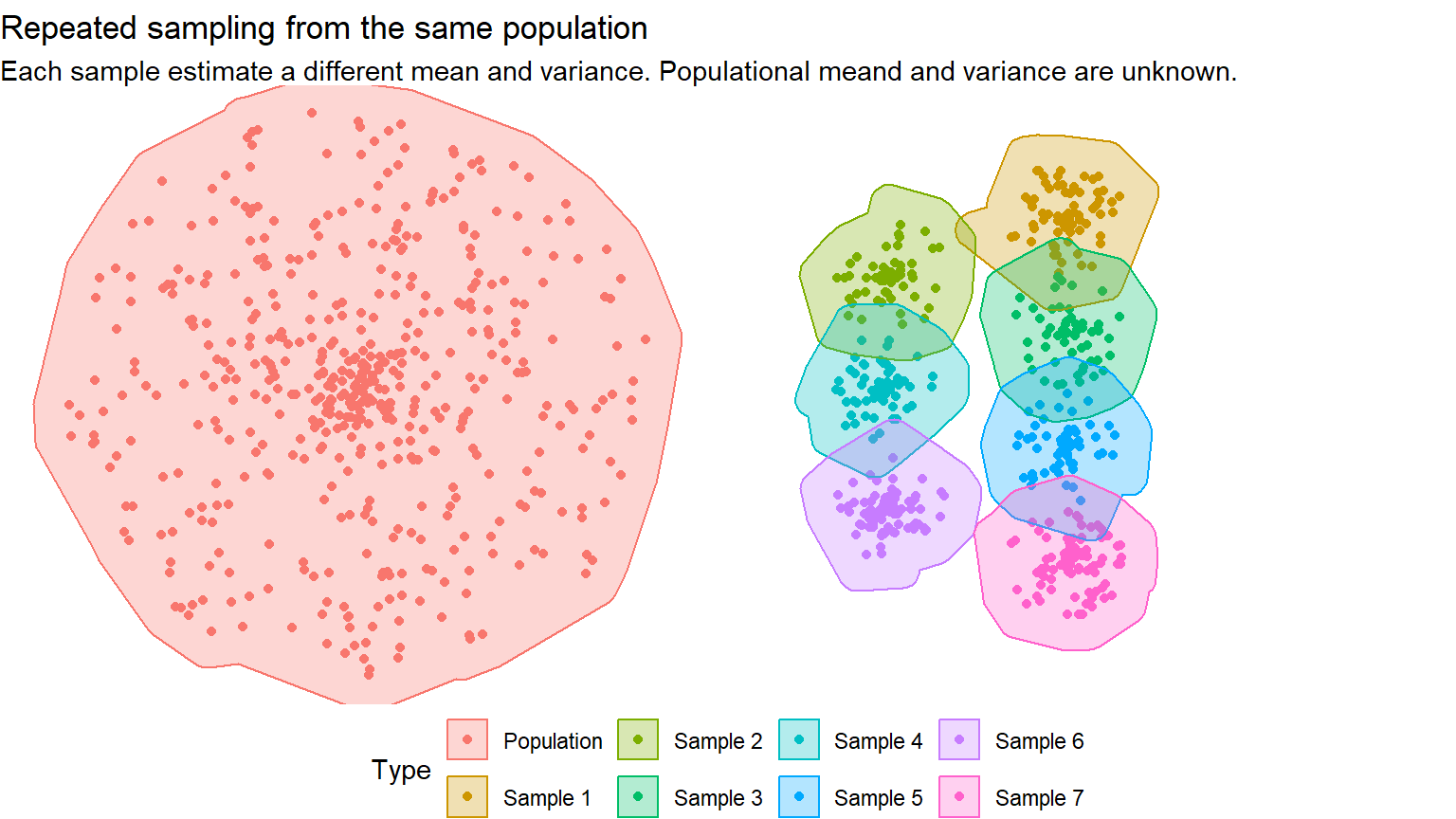
  • we never have the entire population

  • instead, we can only derive (random) samples

  • Therefore, absolute estimates of the population’s parameters (slope and intercept) are insufficient.

    • We need to perform …

    • Hypothesis testing!

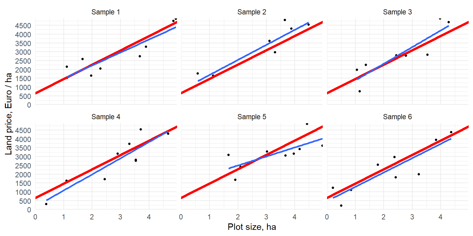
To illustrate this, let us follow-up on the simulated population and derive 6 random samples of 9 observations in each sample.

Sample variation

population regression line is in red and estimated regression line is in blue
Regression: Inference

fit0 <- lm(value ~ area, land_pop)
summary(fit0)
#> Coefficients:
#>             Estimate Std. Error t value Pr(>|t|)    
#> (Intercept) 656.4388     0.7503   874.9   <2e-16 ***
#> area        810.8136     0.2574  3150.0   <2e-16 ***
#> ---
#> Signif. codes:  0 ‘***’ 0.001 ‘**’ 0.01 ‘*’ 0.05 ‘.’ 0.1 ‘ ’ 1
#> 
#> Residual standard error: 515 on 1999998 degrees of freedom
#> Multiple R-squared:  0.8322, Adjusted R-squared:  0.8322 
#> F-statistic: 9.922e+06 on 1 and 1999998 DF,  p-value: < 2.2e-16

\(H_0:\beta = 0\)

\(H_1:\beta \neq 0\)

\(t = {\hat{\beta}}/{se_{\hat\beta}}\)

\(t^* = c_{df, \, 1 - \alpha /2}\)

\(df = n - k\) with \(n\) number of observations and \(k\) number of regressors \(k = 2\) (one for the intercept and one the slope).

  • Reject \(H_0\), when

    • \(|t| > t^*\), or

    • \(\text{p-value} < 0.05\), or

    • \({\hat{\beta}}/{se_{\hat\beta}} > 2\) (rule of thumb).

  • Fail to reject \(H_0\) otherwise.

Regression: Goodness of Fit

fit0 <- lm(value ~ area, land_pop)
summary(fit0)
#> Coefficients:
#>             Estimate Std. Error t value Pr(>|t|)    
#> (Intercept) 656.4388     0.7503   874.9   <2e-16 ***
#> area        810.8136     0.2574  3150.0   <2e-16 ***
#> ---
#> Signif. codes:  0 ‘***’ 0.001 ‘**’ 0.01 ‘*’ 0.05 ‘.’ 0.1 ‘ ’ 1
#> 
#> Residual standard error: 515 on 1999998 degrees of freedom
#> Multiple R-squared:  0.8322, Adjusted R-squared:  0.8322 
#> F-statistic: 9.922e+06 on 1 and 1999998 DF,  p-value: < 2.2e-16

Explanatory power of the model:

  • R-squared

R-squared: measures the fraction of variance in the dependent variable that is explained by the independent variable.

Adjusted R-squared: accounts for the number of independent variables, usually decreasing compared to the R-squared, when we add irrelevant independent variables.

Key Takaway concepts

  • Regression coefficients: an intercept and a slope

  • Interpretation of the regression coefficients

  • Statistical inference about the regression coefficients

  • Fitted (predicted) values

  • Error terms

  • Adjusted R squared.

Self-study: Simple Linear Regression Examples

Review examples below at home:

  • Discuss how would you interpret the coefficients?

Example 1

Comment on (1) what relationship is measured by this regression? (2) what are the interpretations of the coefficients?

  • \(\beta_0\) indicates the expected level of \(yield\) (in the units of \(yield\) ) given zero level of \(fertilizer\) application given that other things (rainfall, land quality, etc.)

  • \(\beta_1\) indicates the expected change in \(yield\) (in the units of \(yield\) ) given one unit change (usually increase, but not always) in \(fertilizer\) application given that other factors remain fixed (rainfall, land quality, etc.)

Example 2
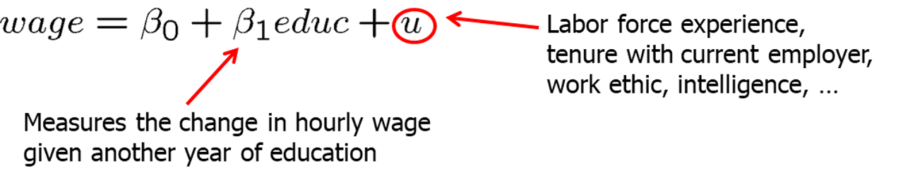
Interpret the slope:

  • With the one year increase in education, average hourly wage increases / (decreases) by \(\beta_1\).

Example 3 Ozone \(O^3\) in stratosphere

The goal of this example is to show that simple linear regression could be used for exposing trends and showing how those trends change significantly after the introduction of a new policy.

  • Ozone \(O^3\) - forms in the stratosphere from oxygen under influence of ultraviolet radiation;
  • The amount of ozone in the atmosphere is very small;
  • Ozone absorbs most of the ultraviolet radiation from the sun;
  • Ozone holes expose humanity to solar radiation.

Background

  • In 1971, James Lovelock had discovered a new compound in the earth’s atmosphere, trichlorofluoromethane, a chlorofluorocarbon (CFC). See: (Lovelock 1971)

  • In 1974 Sherwood Rowland and Mario Molina (Molina and Rowland 1974) discovered the mechanism how CFC gases damage the ozone layer by photolysis. (In 1995 together with Paul Crutzen they were awarded a 1995 Nobel Prize in Chemistry)

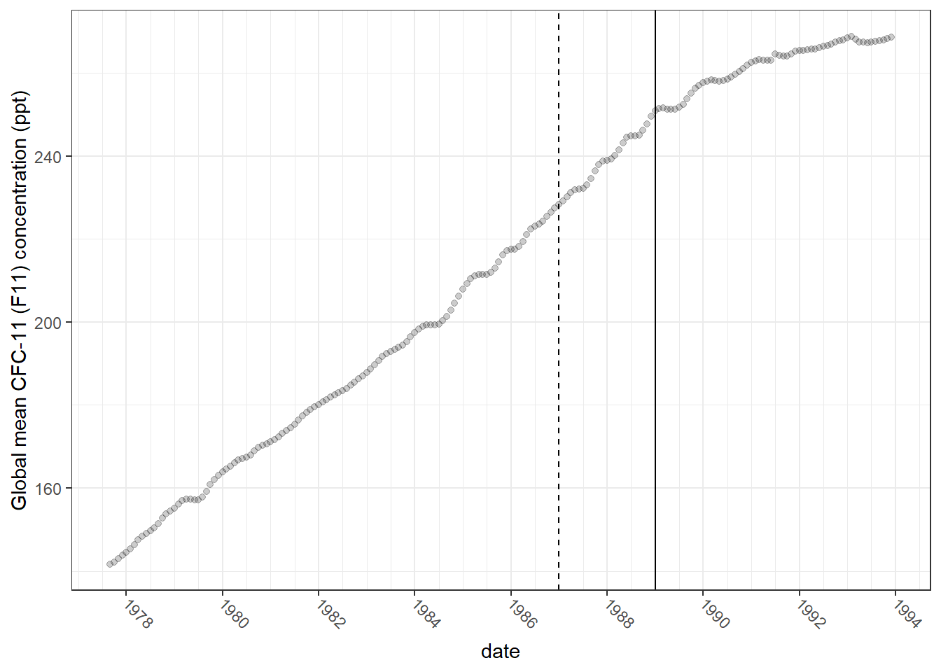
  • In 1987, The Montreal Protocol was accepted by 191 countries aiming to reduce the levels of ozone depleting substances (ODSs) in the atmosphere.

  • It took humanity only 14 years to bridge scientific finding with the global policy.

The problem:

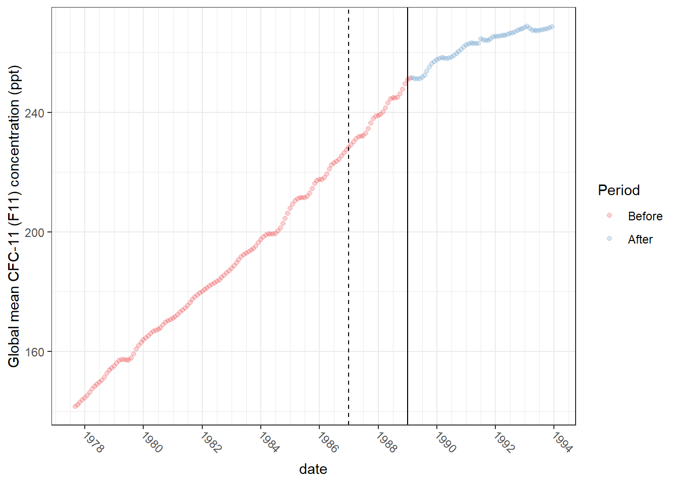
Let us establish a causal effect between the Montreal Protocol and the global CFC-11 emissions/concentration.

CFC-11 content in the atmosphere

To establish a causal relationship,

we can:

  • split data into Before and After The Montreal Protocol;

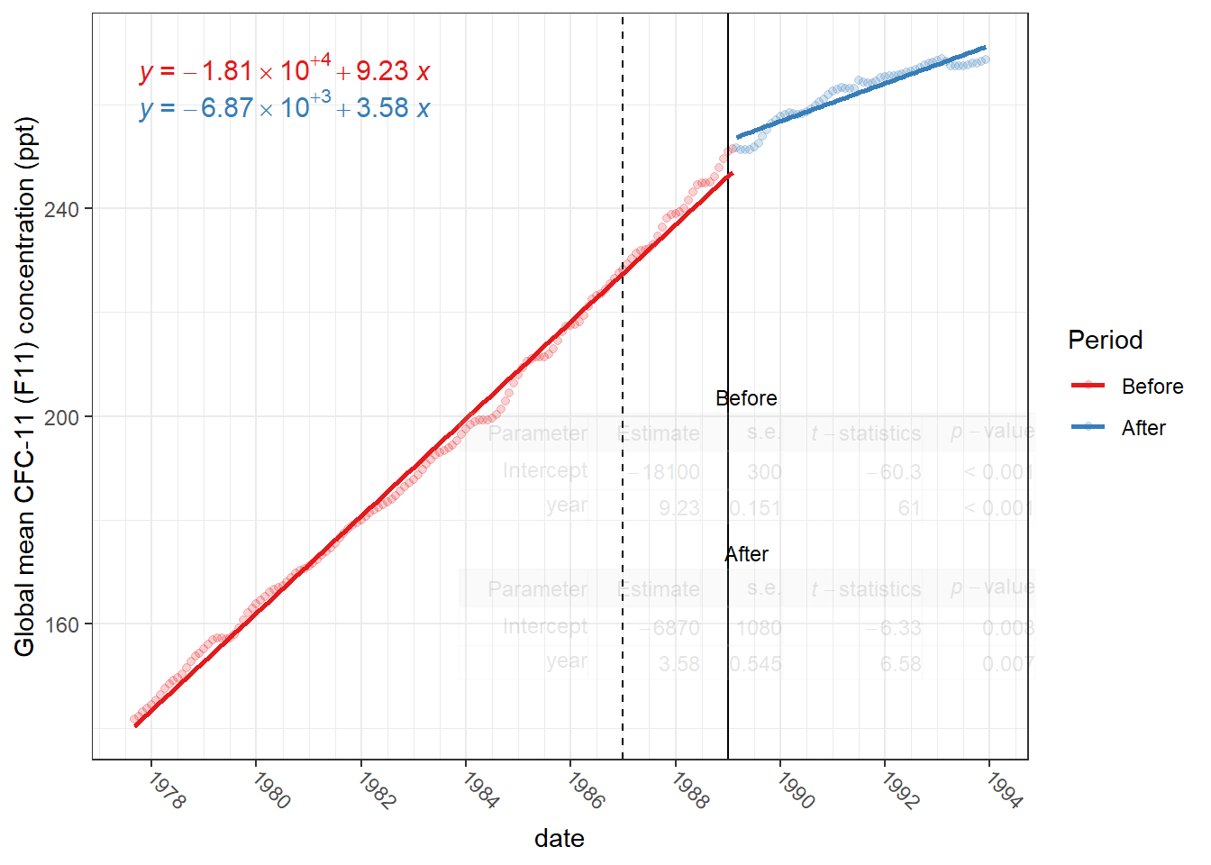
  • fit two separate simple regressions: \(\text{CFC-11} = \hat \beta_0 + \hat \beta_1 \cdot \text{year} + \hat u\)

Why Ceteris Paribus is satisfied here?

  • There are no other factors which could have affected the CFC-11 emissions but the Montreal Protocol.

  • Technology change, although endogenous, has forced to reduce CFC-11 emissions due to the Protocol.

CFC-11 content over time (Monthly averages)
Results of the SLR (1): Coefficients values
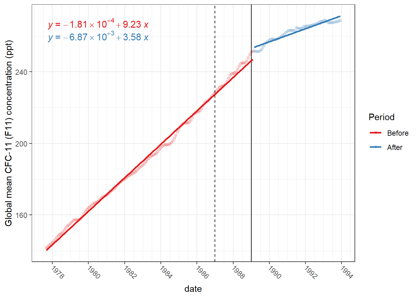
Results of the simple regression (2)
Multiple regression

Multiple Linear Regression vocabulary

Regression equation:

\[y = \hat {\beta}_{0} + \hat {\beta}_{1}x_1 + \hat {\beta}_{2}x_2 + \hat {\beta}_{3}x_3 + \cdots + \hat {\beta}_{k}x_k + \hat u\]

  • \(y\) the dependent variable;

  • \(x_1, x_2, x_3, \cdots x_k\) the independent variables from the set \(k\);

  • \(\hat {\beta}_{0}\) - intercept (constant term);

  • \(\hat {\beta}_{1}\), \(\hat {\beta}_{2}\), \(\hat {\beta}_{k}\) - coefficients / parameters associated with \(x_1\), \(x_2\), … \(x_k\);

Multiple Linear Regression vocabulary (cont.)

After we estimate the regression equation and obtain our estimates \(\hat {\beta}_{0}, \hat {\beta}_{1}, \hat {\beta}_{2}, \cdots, \hat {\beta}_{k}\) we can calculate:

\(\hat y\) fitted of predicted value or the dependent variable and \(\hat u\) error terms

\[\hat y = \hat {\beta}_{0} + \hat {\beta}_{1}x_1 + \hat {\beta}_{2}x_2 + \hat {\beta}_{3}x_3 + \cdots + \hat {\beta}_{k}x_k\]

\[\hat u = y - \hat y\]

Motivation befind MLR

  • To incorporate more explanatory factors into a model;

  • Explicitly hold fixed (some) other factors;

  • Allow for more flexible functional forms;

  • To correct the selection bias problem in the absence of (poor quality of) the RCT;

  • To establish the ceteris paribus in observational data;

Interpretation

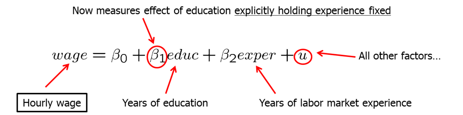
  • The multiple linear regression shows the effect of each variable, holding other explanatory variables fixed;

We assume that all unobserved factors do not change if the explanatory variables are changed.

Example 1. Wage equation
Example 2. Average test scores and spending

Example 3. CEO salary, sales and CEO tenure

  • Model assumes a constant elasticity relationship between CEO salary and the sales of his or her firm.

  • Model assumes a quadratic relationship between CEO salary and his or her tenure with the firm.

Mechanics

\[y = \hat {\beta}_{0} + \hat {\beta}_{1}x_1 + \hat {\beta}_{2}x_2 + \hat {\beta}_{3}x_3 + \cdots + \hat {\beta}_{k}x_k + \hat u\]

  1. MLR uses the Ordinary Least Squares (OLS) method to estimate regression parameters \(\beta\).

    • Such parameters \(\beta\) are found that the sum of squared errors is minimal.
  2. As any estimate of \(\beta\) is based on a sample, we need to relay on the inference to test a hypothesis about the true coefficients in the population.

Example MLR (1). Effect of fuel taxes on petrol consumption

We use data on motor fuel consumption and related variables, for the year 2001. Each observation represents a state in the United States. (based on the data from Weisberg (2005)). Variables are:

  • \(Tax\) : Gasoline state tax rate, cents per liter
  • \(Dlic\) : The number of licensed drivers per 1000 population over the age of 16;
  • \(Income\) : in 1000 USD Per capita personal income (year 2000)
  • \(Miles\) : Miles of Federal-aid highway miles in the state
  • \(Fuel\) : Gasoline consumption per capita (liter)

1. Problem formulation

How do fuel taxes affect gasoline consumption?:

2. Regression model and hypothesis

Write a regression equation:

\[Fuel = \hat\beta_0 + \hat\beta_1 Tax + \hat\beta_2 Dlic + \hat\beta_3 Income + \hat\beta_4 Miles + \hat{u}\]

Discuss, what effects can we expect from change in each variable \(x\) on \(y\)?

Hypotheses:

  • \(\hat\beta_0\) \(>0\) because on average some consumption should occur
  • \(\hat\beta_1\) \(<0\) taxes make flue more expensive leading people to consume less
  • \(\hat\beta_2\) \(>0\) more people with driving licences increase consumption of flue
  • \(\hat\beta_3\) \(>0\) higher income relaxes budget constraints allowing to drive more
  • \(\hat\beta_4\) \(>0\) a larger road network makes people drive more

Exploratory data analysis (1)

rowname mean sd median skew kurtosis se
Tax 20.15 4.54 20.00 -0.67 0.55 0.64
Dlic 903.68 72.86 909.07 -0.30 0.31 10.20
Income 28.40 4.45 27.87 0.62 -0.04 0.62
logMiles 10.91 1.03 11.28 -1.43 1.92 0.14
Fuel 613.13 88.96 626.02 -0.88 2.09 12.46

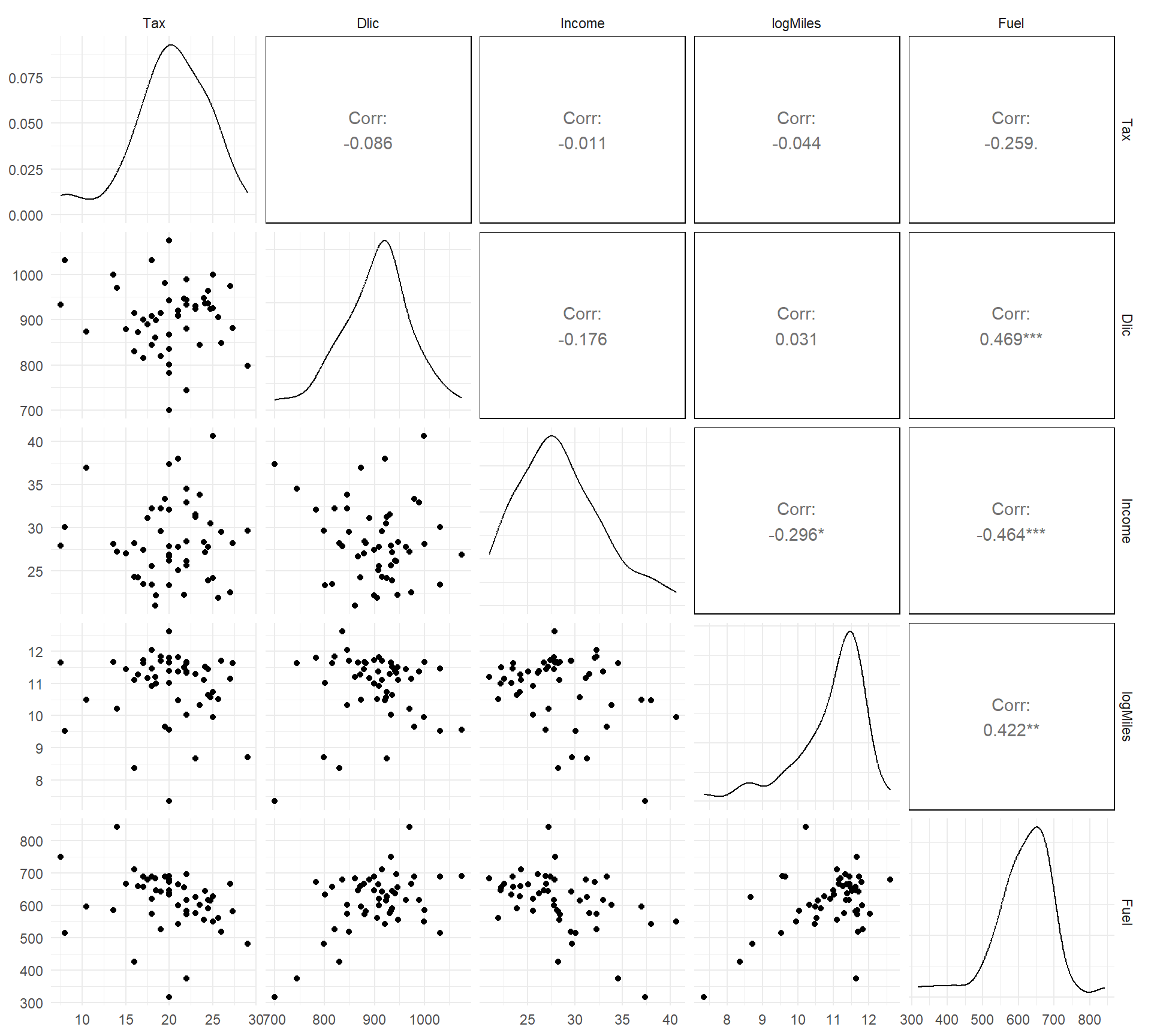
Variable of interest: Tax.

Outcome variable: Fule.

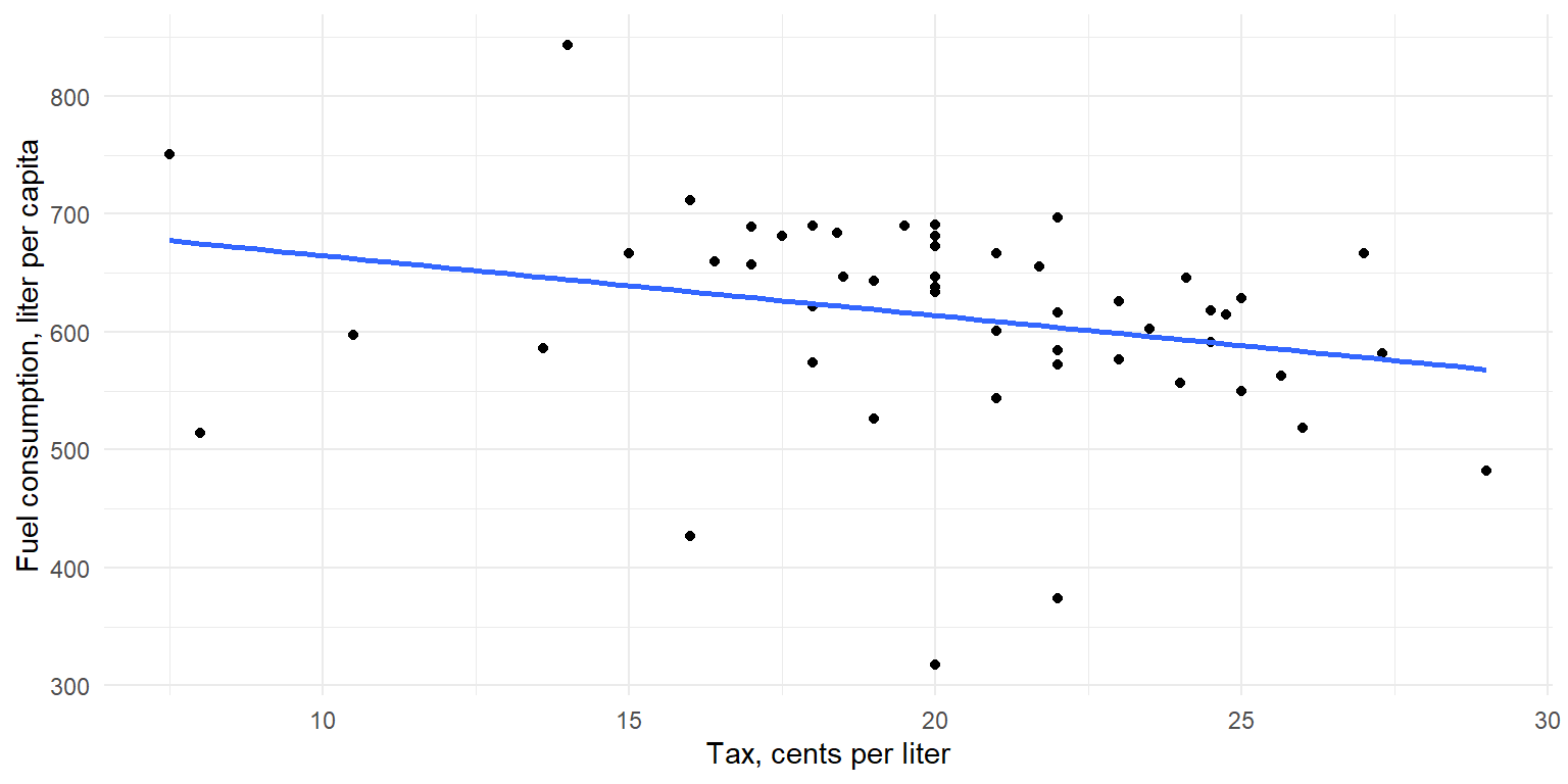
What kind of relationship exists between Tax and Fuel?
Exploratory data analysis (2)

What kind of relationship exists between Tax and Fuel?
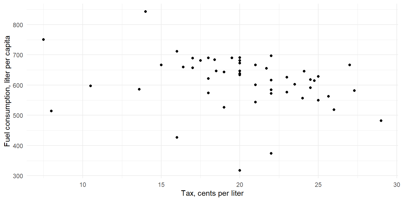
4. Estimating a Simple Linear Reg.

fit_fule_0 <- lm(Fuel ~  Tax, fule_cons)
summary(fit_fule_0)
# Coefficients:
#             Estimate Std. Error t value Pr(>|t|)    
# (Intercept)  715.485     55.770  12.829   <2e-16 ***
# Tax           -5.078      2.701  -1.881    0.066 .  

What does it show?

  • The estaimted effect of taxes is -5.1.
    • A unit change in tax level (1 cent increase in taxes per liter)
    • reduces fuel consumption by 5.1 liters per person
    • assuming all other factors are fixed.
  • However, p-value > 0.05. The same effect of taxes may not hold for the population.
  • Is this the true causal effect? Is there the Ceteris Paribus?
  • NO! We do not control for other things!

4. Estimating the Multiple Linear Regression

Multiple linear regression helps to reveal the true causal effect of Tax by

  • controlling all other things

  • making them equal when the tax changes by one unit

fit_fule_1 <- lm(Fuel ~  Tax + Dlic + Income + logMiles, fule_cons)
summary(fit_fule_1)
# Coefficients:
#             Estimate Std. Error t value Pr(>|t|)    
# (Intercept) 154.1928   194.9062   0.791 0.432938    
# Tax          -4.2280     2.0301  -2.083 0.042873 *  
# Dlic          0.4719     0.1285   3.672 0.000626 ***
# Income       -6.1353     2.1936  -2.797 0.007508 ** 
# logMiles     26.7552     9.3374   2.865 0.006259 ** 

6. Inspecting and interpreting the results

Here we need to:

  • perform the HT about estimated coefficients;

  • interpretation of their economic meaning;

  • compare estimates with ex-ante expectations.

The Intercept

fit_fule_1 <- lm(Fuel ~  Tax + Dlic + Income + logMiles, fule_cons)
summary(fit_fule_1)
# Coefficients:
#             Estimate Std. Error t value Pr(>|t|)    
# (Intercept) 154.1928   194.9062   0.791 0.432938    
# Tax          -4.2280     2.0301  -2.083 0.042873 *  
# Dlic          0.4719     0.1285   3.672 0.000626 ***
# Income       -6.1353     2.1936  -2.797 0.007508 ** 
# logMiles     26.7552     9.3374   2.865 0.006259 **
  • Positive but insignificant at the 5% level. (p-value = 0.432).

  • Contradicts our ex-ante hypothesis about some basic level of fuel consumption;

  • Suggests that the absence of a road network could drive fuel consumption to zero.

The Slope of Taxes

fit_fule_1 <- lm(Fuel ~  Tax + Dlic + Income + logMiles, fule_cons)
summary(fit_fule_1)
# Coefficients:
#             Estimate Std. Error t value Pr(>|t|)    
# (Intercept) 154.1928   194.9062   0.791 0.432938    
# Tax          -4.2280     2.0301  -2.083 0.042873 *  
# Dlic          0.4719     0.1285   3.672 0.000626 ***
# Income       -6.1353     2.1936  -2.797 0.007508 ** 
# logMiles     26.7552     9.3374   2.865 0.006259 **
  • Negative and significant at the 5% level (p-value = 0.043).

  • One cent increase in taxes per liter causes flue consumption to reduce by -4.2 liter per capita, given that all other factors remain fixed.

    • Note: \(Tax\) Gasoline state tax rate, cents per liter and \(Fuel\) Gasoline consumption per capita (liter)
  • This is in line with our ex-ante hypothesis.

The Slope of Income

Note: \(Income\) in 1000 USD Per capita personal income (the year 2000)

fit_fule_1 <- lm(Fuel ~  Tax + Dlic + Income + logMiles, fule_cons)
summary(fit_fule_1)
# Coefficients:
#             Estimate Std. Error t value Pr(>|t|)    
# (Intercept) 154.1928   194.9062   0.791 0.432938    
# Tax          -4.2280     2.0301  -2.083 0.042873 *  
# Dlic          0.4719     0.1285   3.672 0.000626 ***
# Income       -6.1353     2.1936  -2.797 0.007508 ** 
# logMiles     26.7552     9.3374   2.865 0.006259 ** 
  • Negative and significant at the 5% level (p-value = 0.043).

  • An increase in income by 1000 USD per person causes fuel consumption to reduce by -6.1 liter per capita, ceteris paribus.

  • This contradicts our ex-ante hypothesis. Why?

The Slope of logMiles

Note: \(logMiles\) is the logarithm of miles. Interpretation differs because this is a level-log transformation

fit_fule_1 <- lm(Fuel ~  Tax + Dlic + Income + logMiles, fule_cons)
summary(fit_fule_1)
# Coefficients:
#             Estimate Std. Error t value Pr(>|t|)    
# (Intercept) 154.1928   194.9062   0.791 0.432938    
# Tax          -4.2280     2.0301  -2.083 0.042873 *  
# Dlic          0.4719     0.1285   3.672 0.000626 ***
# Income       -6.1353     2.1936  -2.797 0.007508 ** 
# logMiles     26.7552     9.3374   2.865 0.006259 ** 
  • Positive and significant at the 5% level (p-value = 0.043).

  • An increase in road network by 1% causes fuel consumption to increase by 26.7/100 (0.26) liter per capita, given ceteris paribus.

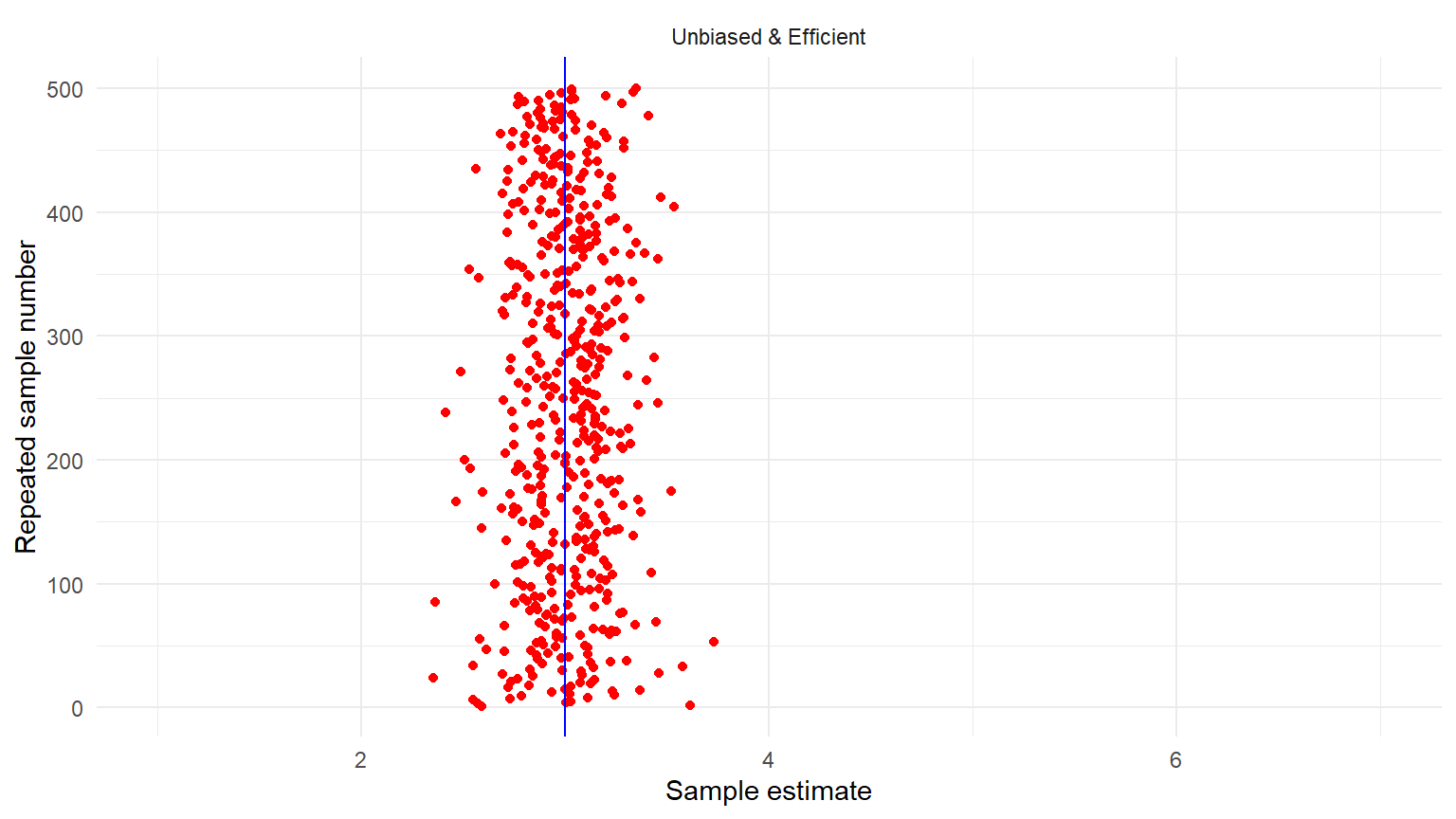
Bias and Efficiency

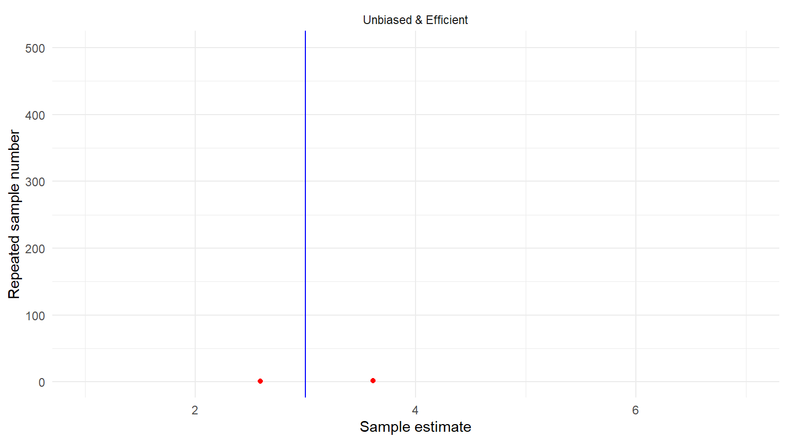
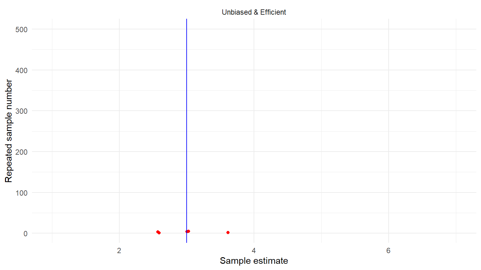
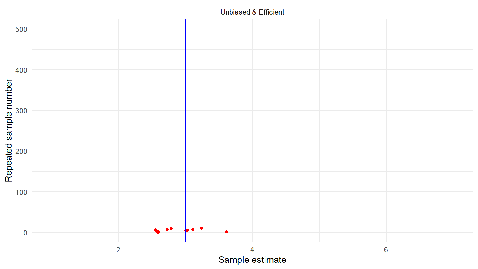
Sampling from the population

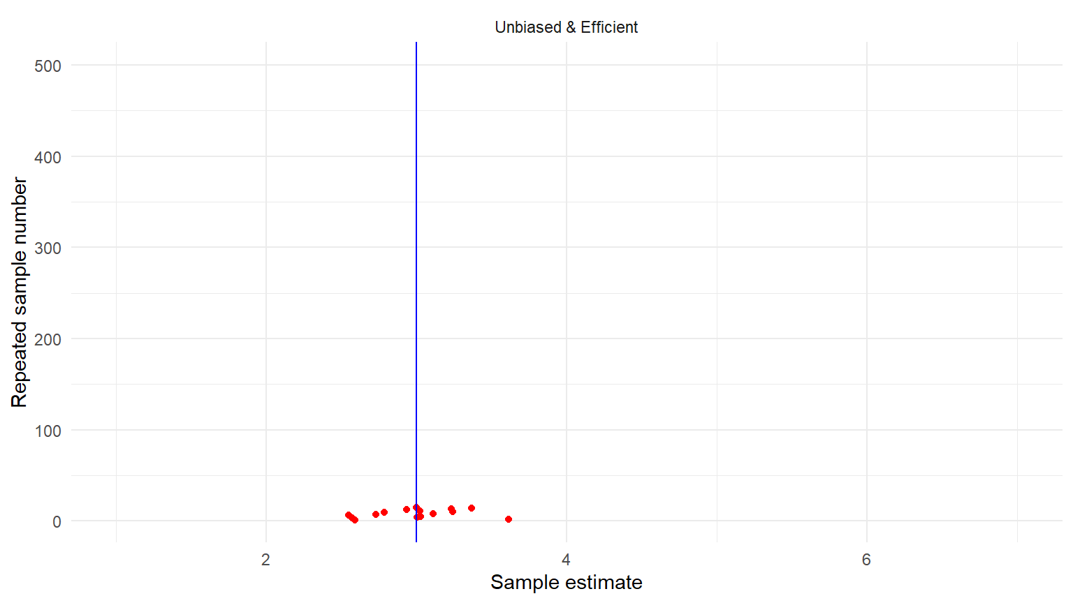
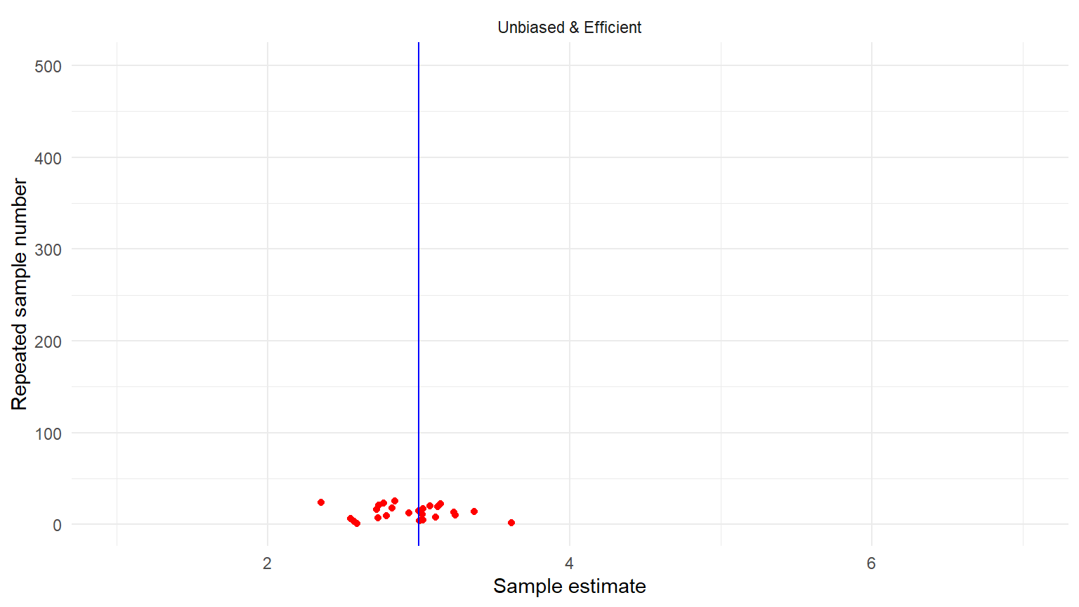
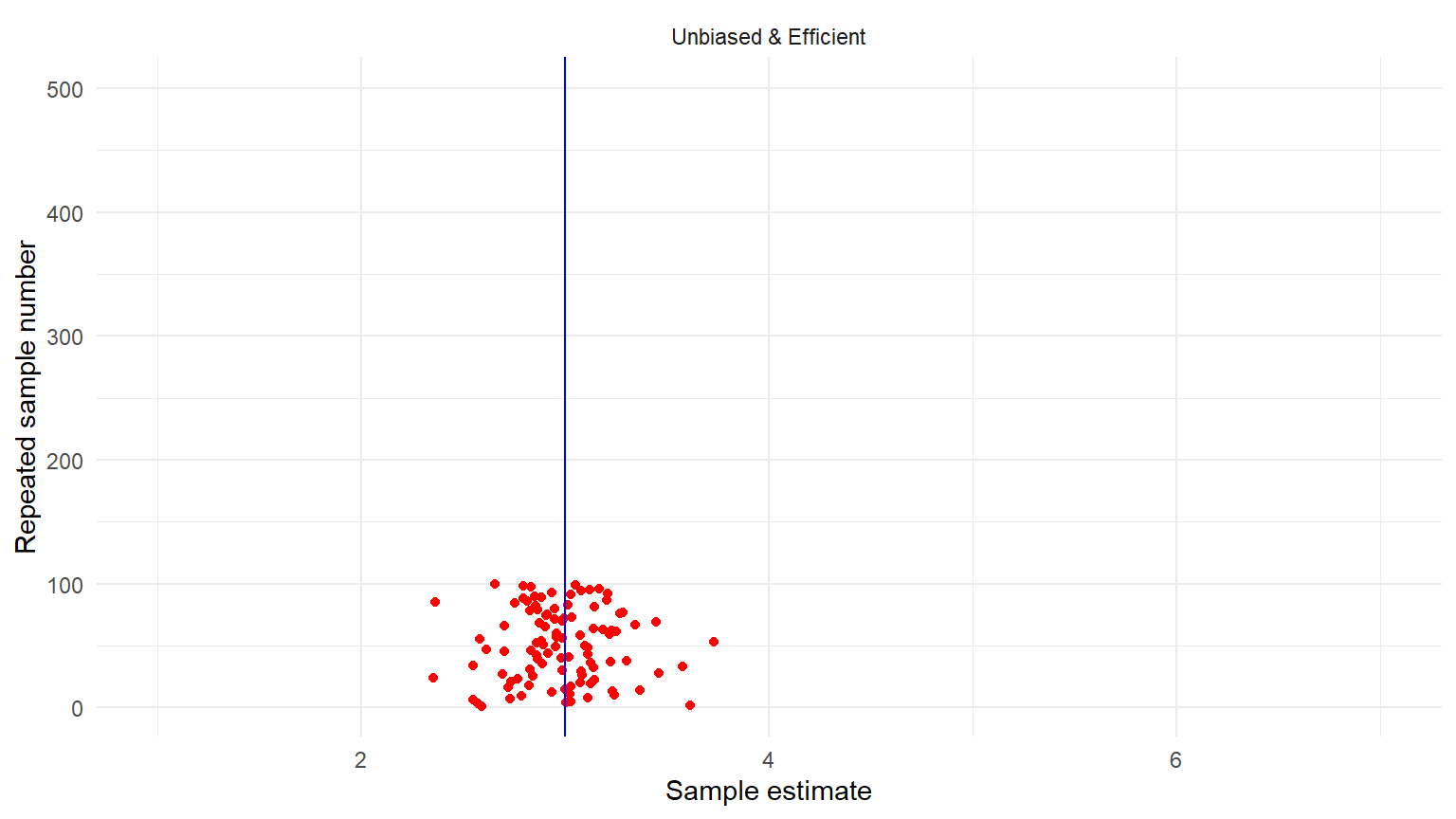
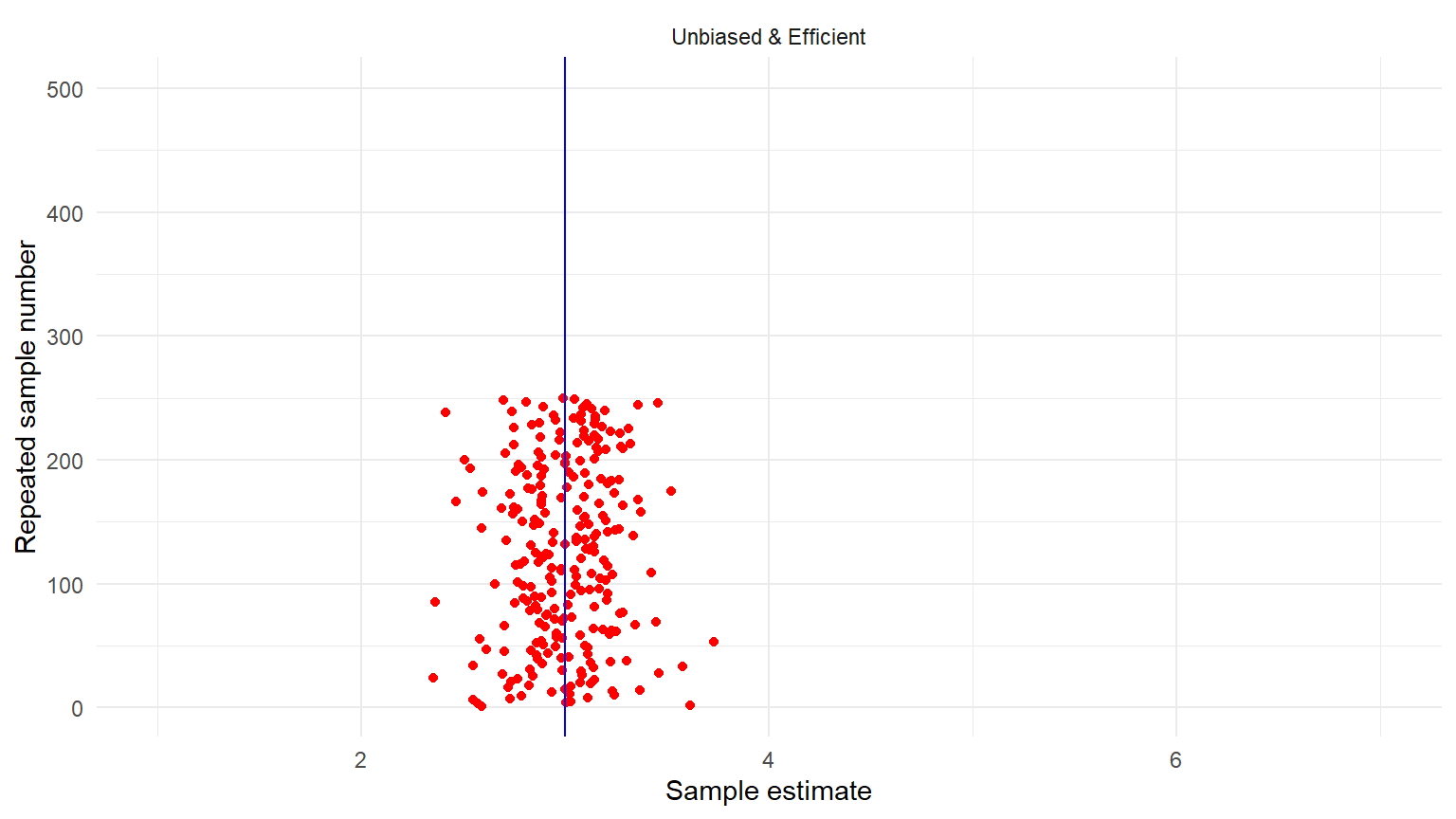
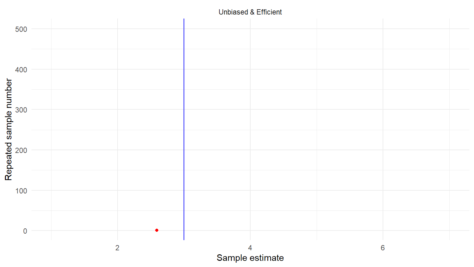
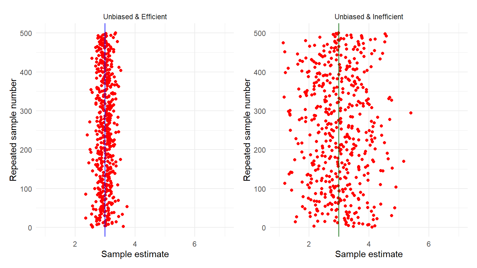
Unbiased and efficient estimates
Unbiased but inefficient
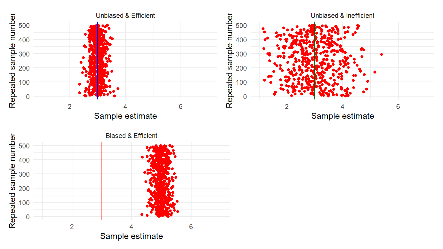
Biased but efficient
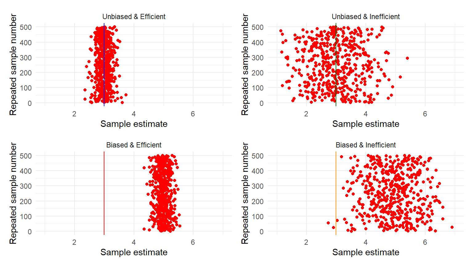
Biased and inefficient
Assumptions of the MLR

exist to ensure that linear regression estimates are unbiased and efficient!

OLS is unbiased. Assumptions 1 to 4 are satisfied:

  1. Linearity
  2. Random Sampling
  3. No Collinearity
  4. No Endogeneity

OLS is unbiased and efficient. Best Linear Unbiased Estimator (BLUE). Assumptions 1 to 5 are satisfied

  1. Homoscedasticity (No Autocorrelation)

OLS is a Classical linear model (CLM). Assumptions 1 to 6 are satisfied

  1. Error Terms Normality

Assumption 1. Linearity

Linearity

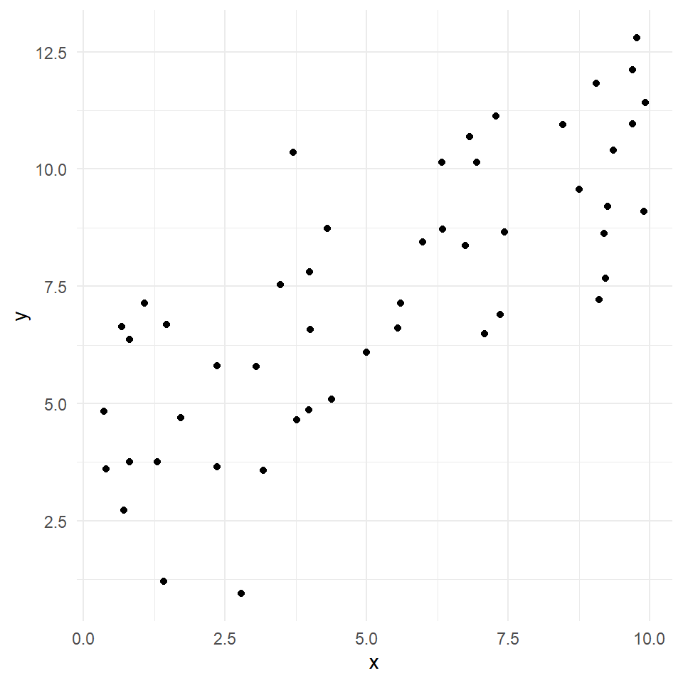
  • the expected value of the dependent variable is a straight-line function of the independent variable

  • If linearity is violated:

    • the estimates are biased and regression is invalid!

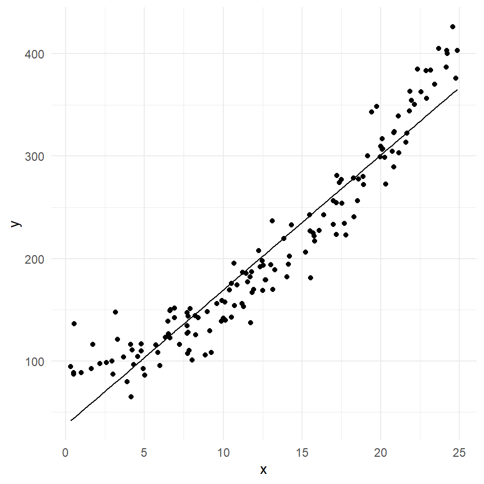
Can we draw a straight line through the dots?
Linearity: detection

To detect non-linearity, we inspect data visually with:

  • Scatter plots of dependent variable \(y\) plotted versus independent variables (\(x\)).

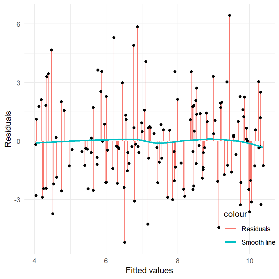
  • Scatter plot of residuals versus predicted/fitted values

Linearity detection (1)

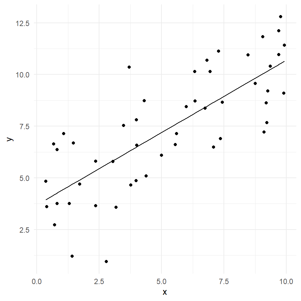
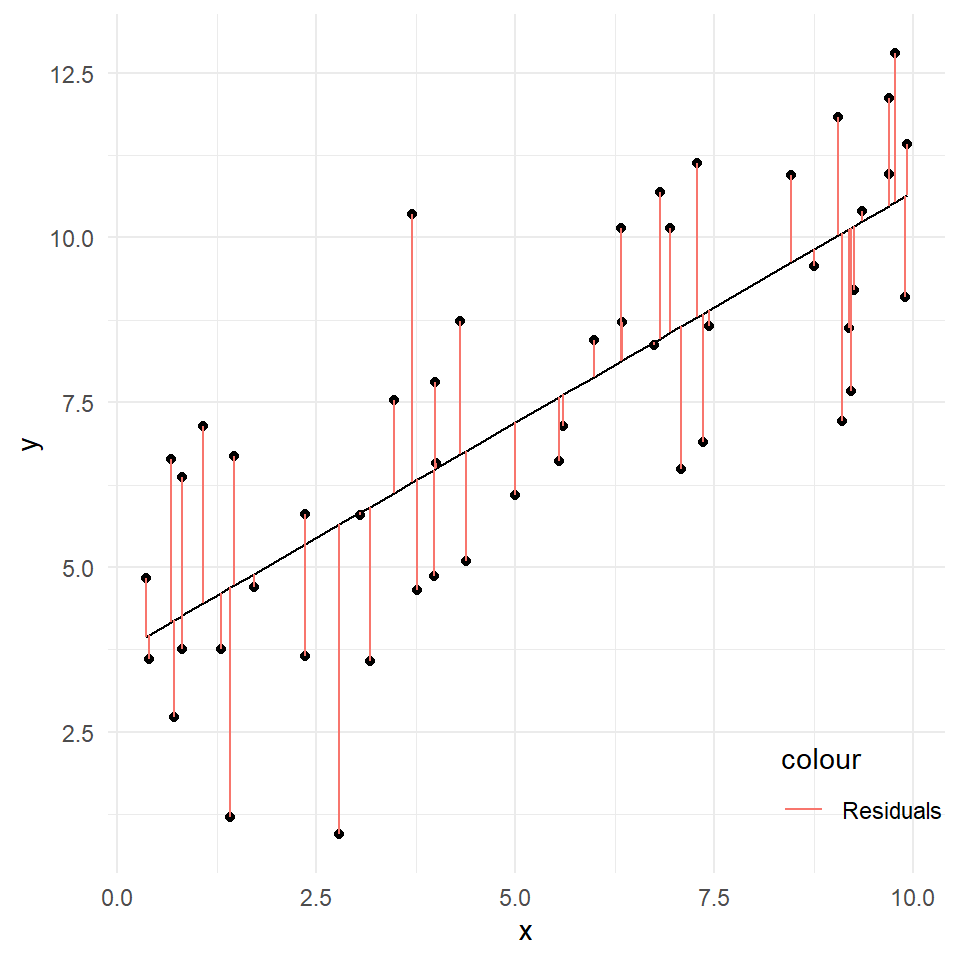
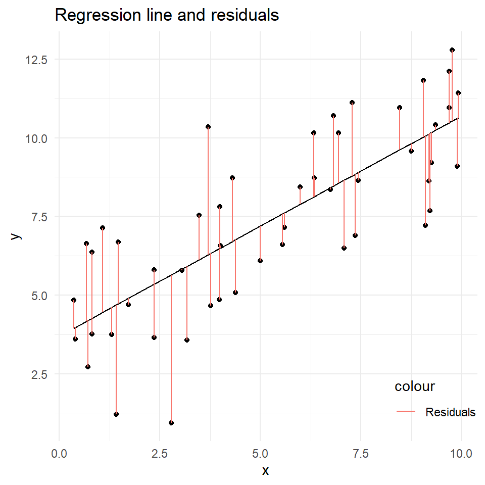
We’ve estimated a regression mode \(Y = \beta_0 + \beta_1 x\) on 50 observations. Results:
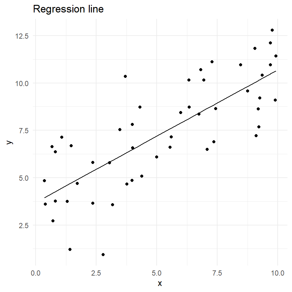
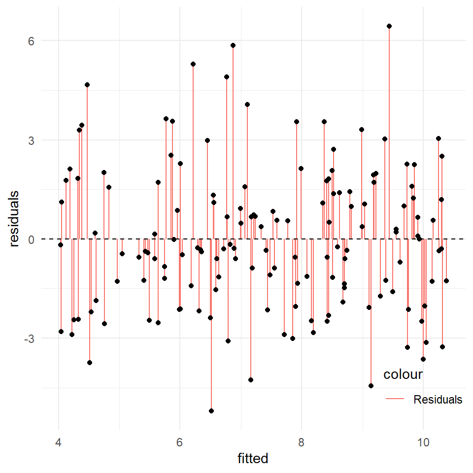
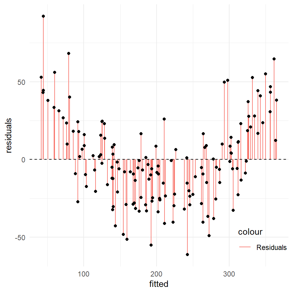
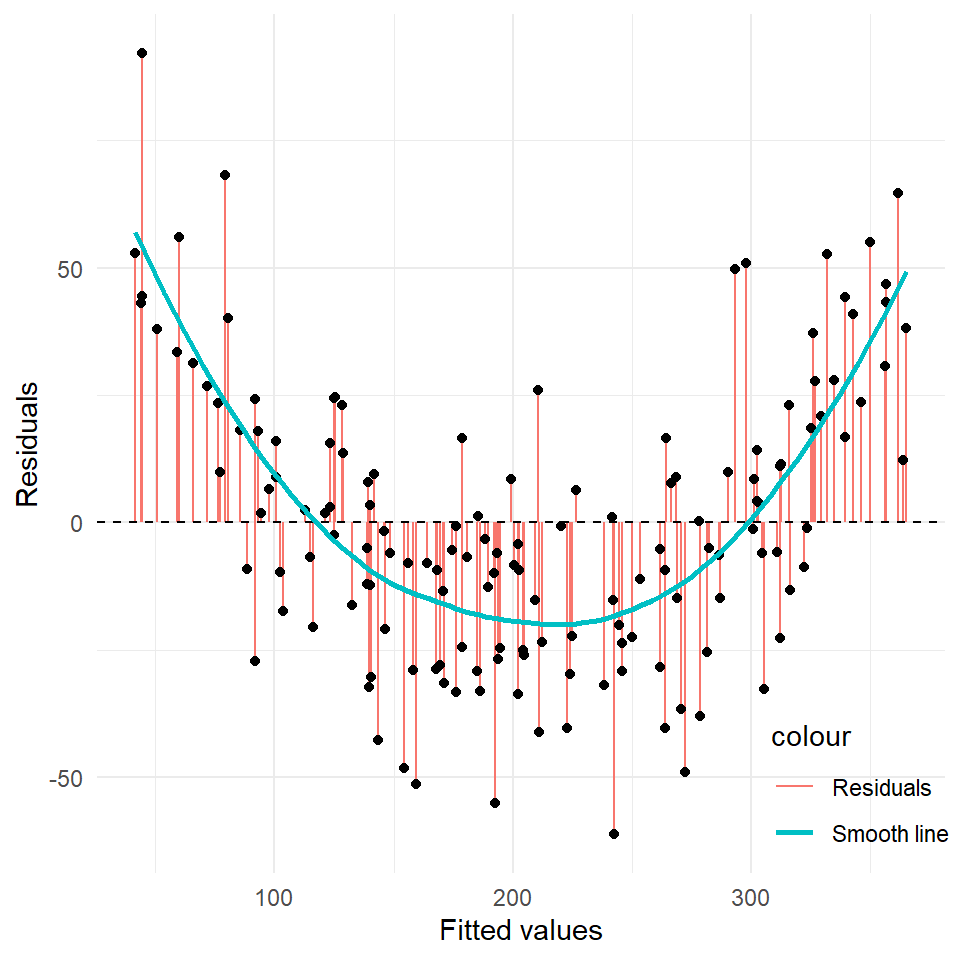
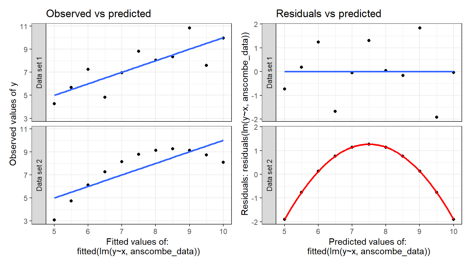
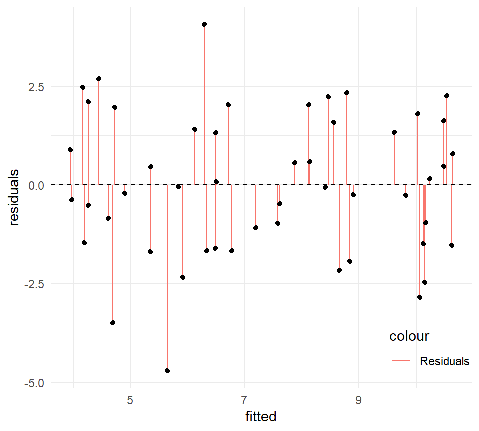
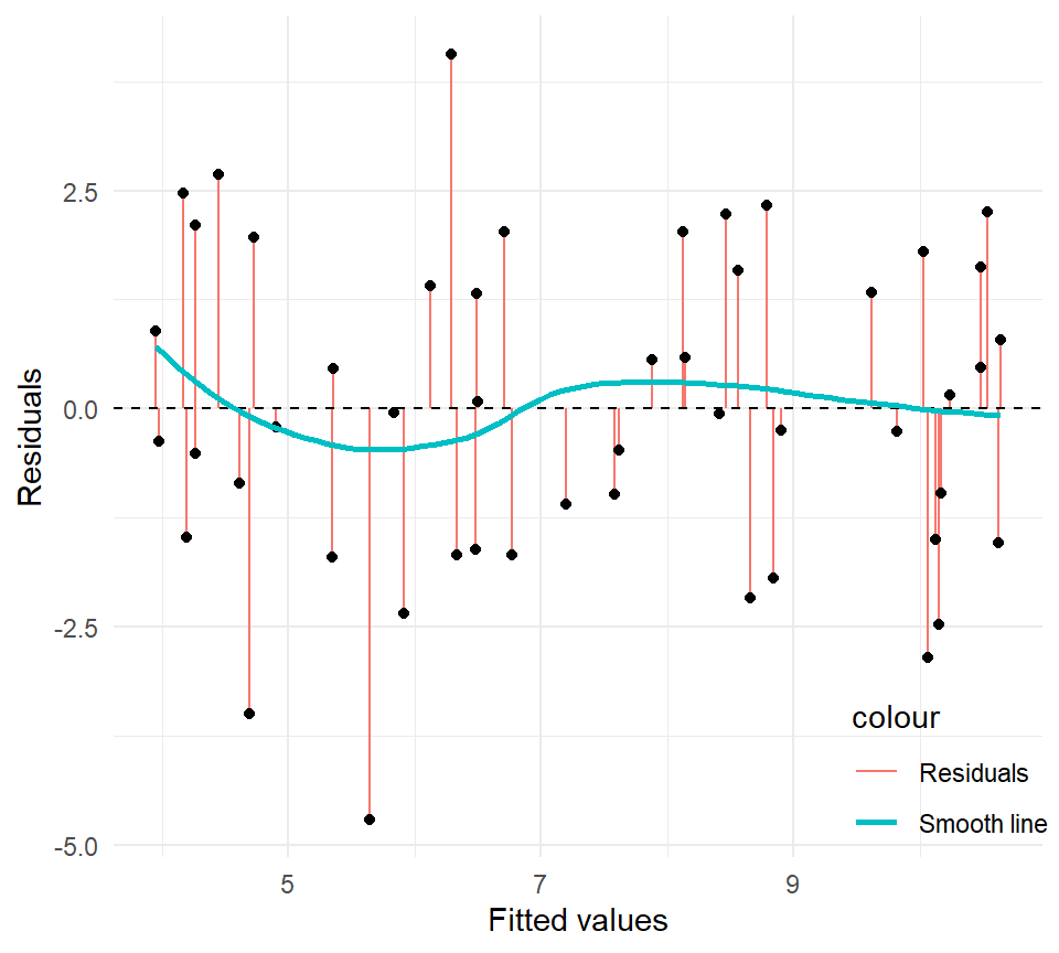
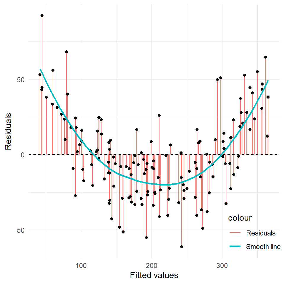
To check nonlinearity, we need to plot fitted values on \(x\) axis and residuals on \(y\) axis.

If we can draw a horizontal line through the dots, we have linearity, if not, we have non-linearity.
Linearity detection (2)

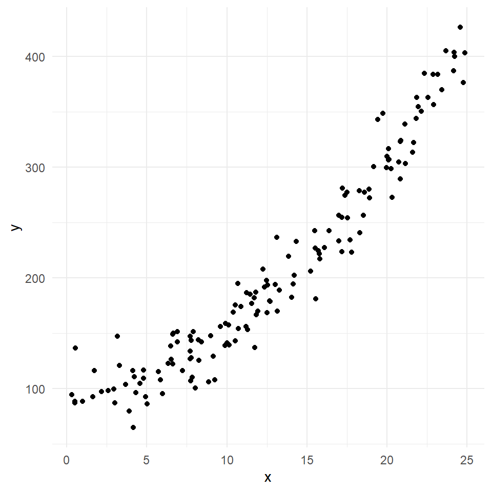
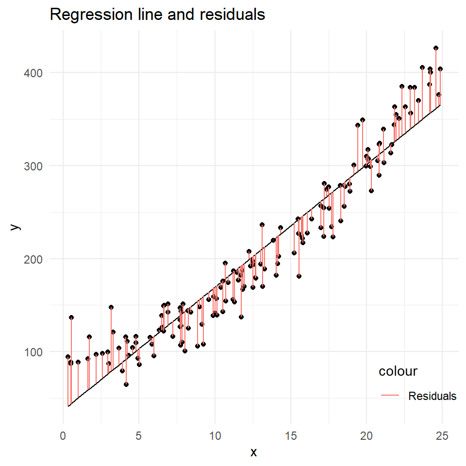
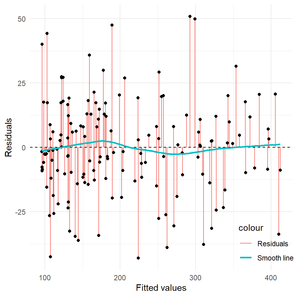
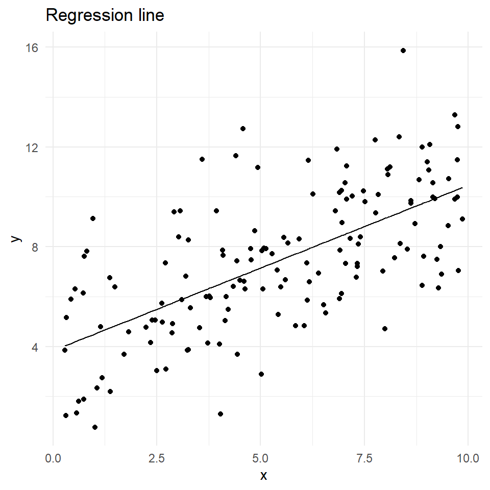
Here we use the same population but increase our sample size to 150 observations. (Small sample size may cause seeming nonliearities).
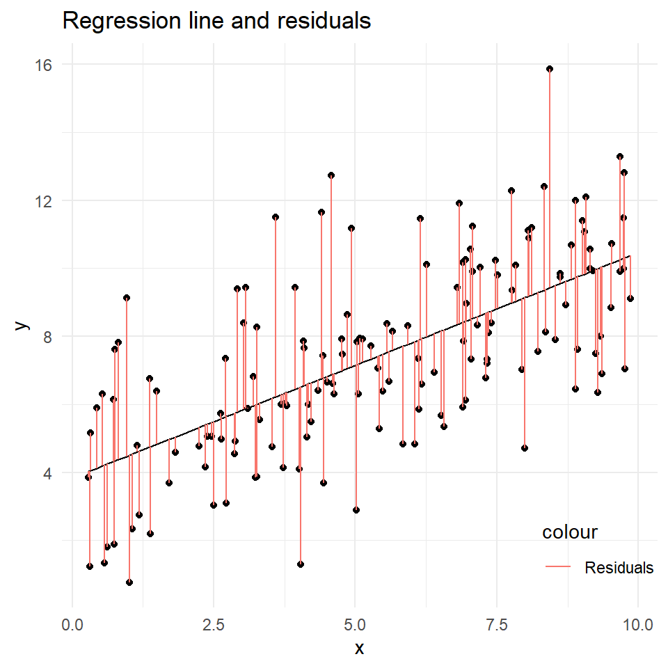
Linearity detection (3)
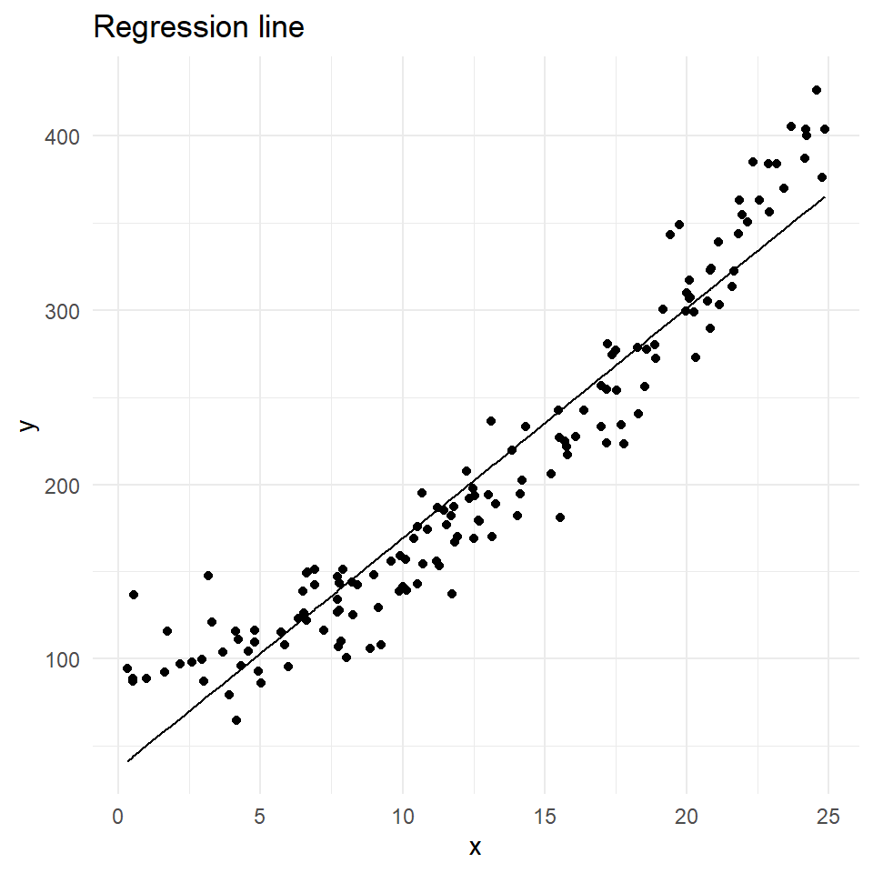
Linearity: resolutions

  1. Functional form: multiple regression and transformation.

  2. (non) linear transformation to the dependent and/or independent variables;

    • does change the way how we must interpret coefficients;
  3. find a different independent variable;

  4. propose a different functional form;

Example of linearity resolution

We had nonlinearity with a simple regression: \(y = \beta_0 + \beta_1x\).
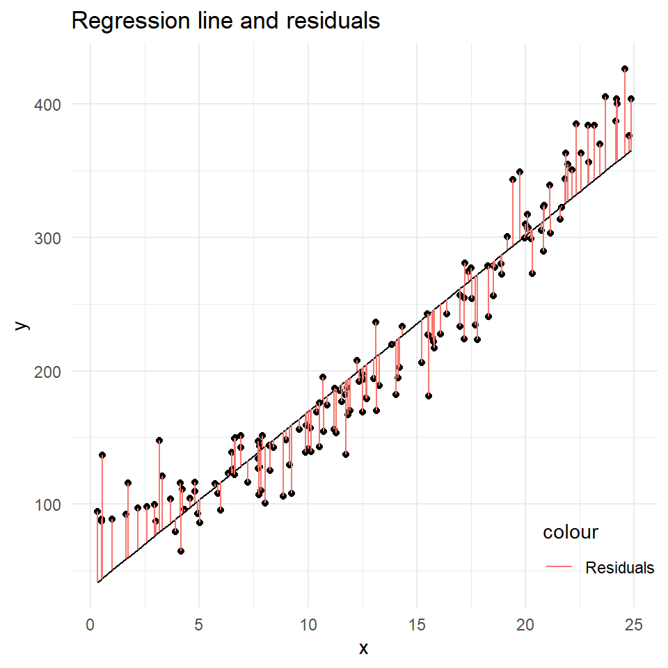
Let us estimate a multiple regression: \(y = \beta_0 + \beta_1 x + \beta_2 x^2\).
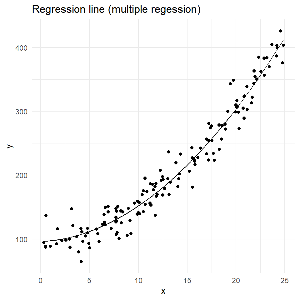
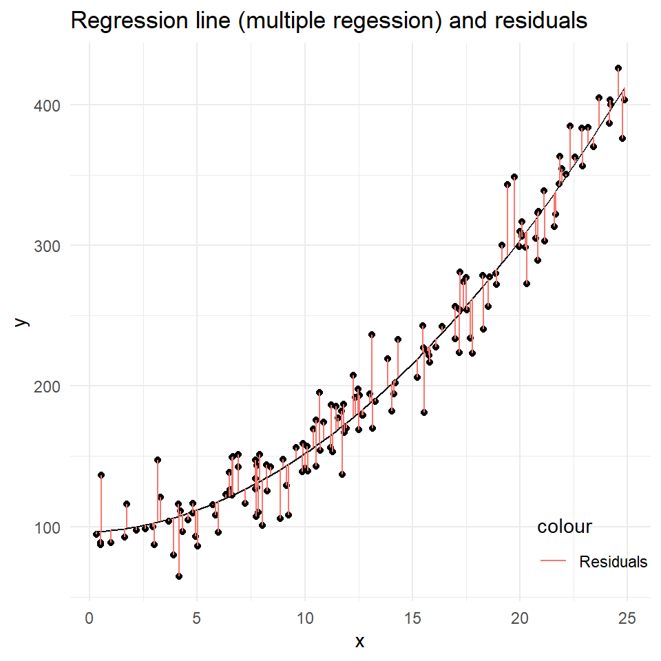
Example of linearity resolution (cont.)

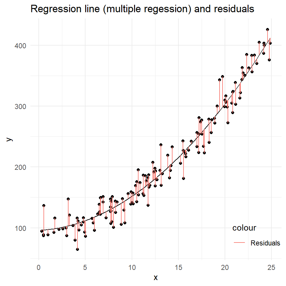
After the linear transformation of \(x\) and multiple regression \(y = \beta_0 + \beta_1x\), our regression line is a curve (non linear).
Residuals vs. Fitted plot also changes:
Common linear transformations

Model Dep. Var. Indep. Var. Interpretation of \(\beta_1\) Interpretation
Level-level \(y\) \(x\) \(\Delta y = \beta_1 \Delta x\) 1 unit change in \(x\) causes \(\beta_1\) units change in \(y\)
Level-log \(y\) \(log(x)\) \(\Delta y = (\beta_1/100)\% \Delta x\) 1 % change in \(x\) causes \(\beta_1/100\) units change in \(y\)
Log-level \(log(y)\) \(x\) \(\% \Delta y = (100\beta_1) \Delta x\) 1 unit change in \(x\) causes \(100 \beta_1\) % change in \(y\)
Log-log \(log(y)\) \(log(x)\) \(\% \Delta y = \beta_1 \% \Delta x\) 1 % change in \(x\) causes \(\beta_1\) % change in \(y\) (elasticity)
  • Power transformation (\(x^2\), \(\sqrt x\)), Box-Cox transformations;

  • Variables normalization to the standard normal distribution;

  • Tailor expansion (Cobb-Douglas, Trans-log)

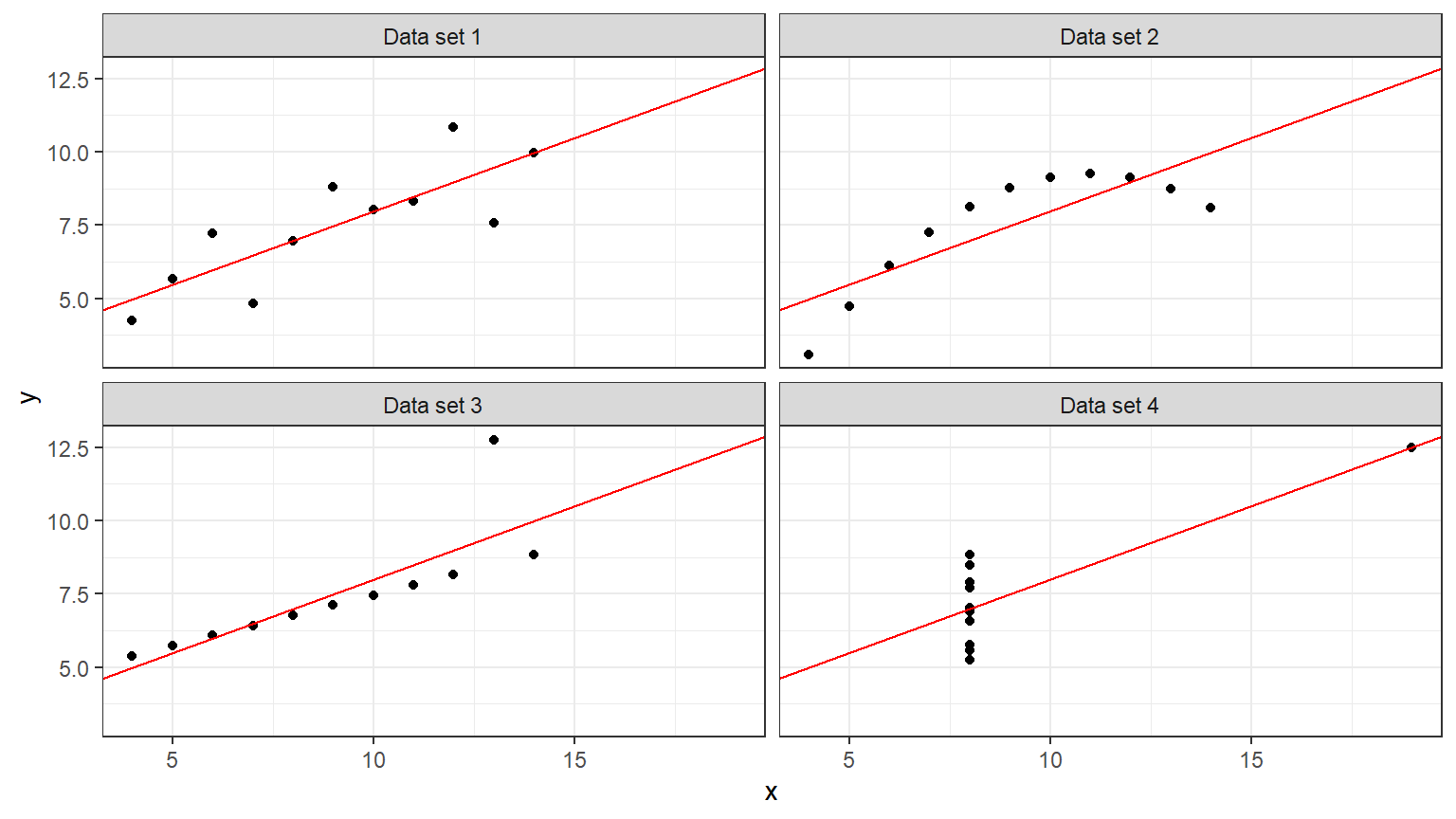
Linearity Example 1: Anscombe quartet

The Anscombe quartet

  • Four data sets of 11 observations each and two variables (x and y).

SLR y on x

Scatter plots

Residuals vs fitted

Takeaways checklist

Key concepts covered in the lecture

Simple linear regression:

  • Regressor and regressand;
  • Fitted values and residuals;
  • OLS method;
  • Estimated coefficients;
  • Interpretation of the slope and the intercept.
  • HT about the regression coefficients.

Ceteris Paribus

  • Establishing Ceteris Paribus without an RCT.
  • Multiple Linear Regression that controls for other things.

Multiple linear regression

  • Coefficients, HT and interpretation.
  • Goodness of fit.
  • Causal meaning.
  • Observed included, not included and unobserved factors.
  • Interpreting coefficients of the MLR.

Assumptions of the regression analysis.

  • Bias and unbiased estimates.
  • Role of assumptions in the bias of the estimates.

Linearity assumption

  • Detection.
  • Implications or why the linearity assumption is important.
  • How to correct the non-linearity (linear transformation).

Self-study: Cradle of the Regression Analysis

  • The term “regression” was coined by Sir Francis Galton, Charles Darwin’s half-cousin, in 1886

    • he was gripped by Darwin’s masterpiece, The Origin of Species.

    • he used “Regression” to prove his points of Eugenics…

Statistics has some dark history…

Paper: Francis Galton, “Regression towards Mediocrity in Hereditary Stature,” Journal of the Anthropological Institute of Great Britain and Ireland, vol. 15, 1886, pages 246–263

Galton’s introduction of regression

  • Galton discovered that the average heights of fathers and sons are linked by a regression equation.

  • the average height of sons is a weighted average of their fathers’ height and the average height in the population from which the fathers and sons were sampled.

First application in causality analysis

  • pioneered by George Udny Yule in “An Investigation into the Causes of Changes in Pauperism in England, Chiefly during the Last Two Intercensal Decades,” Journal of the Royal Statistical Society, vol. 62, no. 2, June 1899, pages 249–295.

  • Student of statistician Karl Pearson (Pearson’s correlation …) and Galton’s protege.

Yule realized that Galton’s regression method could be extended to include many variables (multiple regression).

George Udny Yule

In an 1899 MLR was used to link the administration of the English Poor Laws in different counties to the likelihood county residents were poor, while controlling for population growth and the age distribution in the county.

  • The poor laws provided subsistence for the indigent, usually by offering shelter and employment in institutions called workhouses.

  • Yule was particularly interested in whether the practice of outdoor relief, which provided income support for poor people without requiring them to move to a workhouse, increased poverty rates by making pauperism less onerous.

  • This is a well-defined causal question much like those that occupy social scientists today.

The past of statistics

Statistics has a dark past.

  • It was used and developed in the disposal of really terrible things like Eugenics.

  • But the world was terrible then.

Nowadays, same statistical methods are fundamental for revealing causal effects as 100 years ago.

  • Yet we apply it for some different causes.

References

Angrist, Joshua D., and Jörn-Steffen Pischke. 2009. Mostly Harmless Econometrics. Princeton University Press. https://doi.org/10.1515/9781400829828.
Angrist, Joshua D., and Jörn-Steffen Pischke. 2014. Mastering’metrics: The Path from Cause to Effect. Princeton University Press.
Lovelock, J. E. 1971. “Atmospheric Fluorine Compounds as Indicators of Air Movements.” Nature 230 (5293): 379–79. https://doi.org/10.1038/230379a0.
Molina, Mario J., and F. S. Rowland. 1974. “Stratospheric Sink for Chlorofluoromethanes: Chlorine Atom-Catalysed Destruction of Ozone.” Nature 249 (5460): 810–12. https://doi.org/10.1038/249810a0.
Ritter, Matthias, Silke Hüttel, Martin Odening, and Stefan Seifert. 2020. “Revisiting the Relationship Between Land Price and Parcel Size in Agriculture.” Land Use Policy 97 (September): 104771. https://doi.org/10.1016/j.landusepol.2020.104771.
Weisberg, Sanford. 2005. Applied Linear Regression. John Wiley & Sons, Inc. https://doi.org/10.1002/0471704091.
Wooldridge, M. Jeffrey. 2020. Introductory Econometrics: A Modern Approach. South-Western. https://www.cengage.uk/shop/isbn/9781337558860.