Week 05. Hypothesis testing II. Central Limit Theorem. T-distribution. Confidence intervals. t-test

Part 1: Statistics and Econometrics. MK68-2024/25

Eduard Bukin

eduard.bukin@agrar.uni-giessen.de

Justus Liebig University Giessen

Institute of Agricultural Policy and Market Research

Content

• t-test with the Conditional Cash Transfers (CCTs)
• Normally distributed population and the confidence intervals
• The Central Limit Theorem (CLT)
• The Confidence Interval
• Application of the t-distribution
• Practice
• Example 1: Effect of a drug on sleep (1)
• Example 2: Travel time difference between treatment and control
• Example 3: Causal effect of treatment on enrollment
• Extra materials (for self-study)
• t-test
• t-scores
• Homework
• References

t-test with the Conditional Cash Transfers (CCTs)

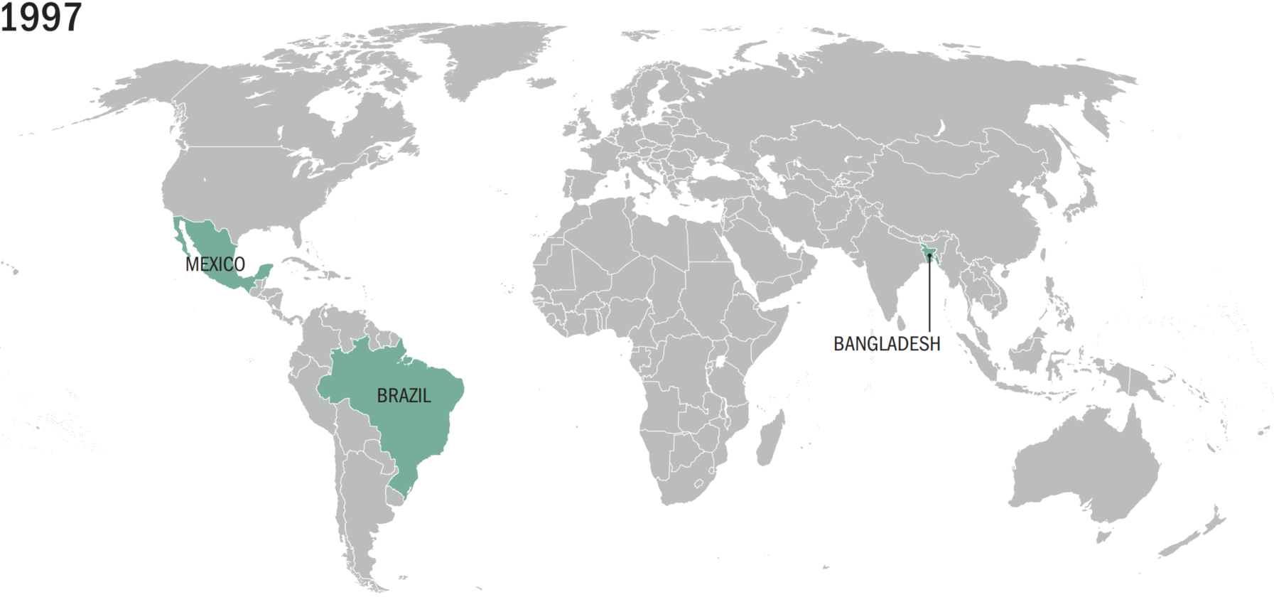
Let us consider an example of CONDITIONAL CASH TRANSFERS’ causal effect on children school enrollment.

See: CH 5. The Impact of CCT Programs on the Accumulation of Human Capital from (Fiszbein et al. 2009).

Conditional Cash Transfers (CCTs)

CCTs are programs that transfer cash on the condition of making pre-specified investments in human capital and children. (Fiszbein et al. 2009, fig. 1)

Cause and Effect

1. Cause / Treatment:

• CCTs (monetary incentive) + Pre-specified conditions

2.a Outcome / Factual

• School enrollment
• in treatment;

2.b Counterfactual

• School enrollment
• in control;

3. ATE: \(\text{Effect} = \text{Factual} - \text{Counterfactual}\)

• \(\text{Average Treatment Effect} = \text{Enrollment Rate Difference}\)

What makes “Difference in Enrollment Rate” a causal effect?

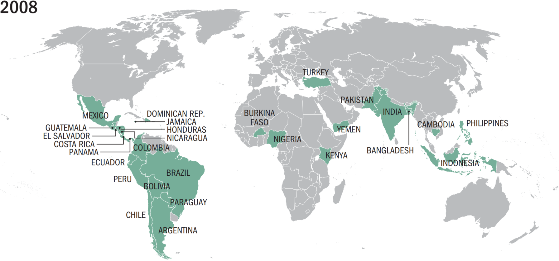
What statistical concepts ensure that the difference in school enrollment between the treatment and control is caused by the treatment?

1. Research Designed with the RCT:

   • Randomization between the Control and Treatment group;

2. the Law of Large Numbers (LLN):

   • Both random groups are equal on average;

3. The RCT + LLN = Ceteris Paribus;

   • All other things are equal between the Control and Treatment groups;

Good controls in the RCT

The control group is a perfect counterfactual when three conditions are met:

1. has the same characteristics, on average, as the treatment group;

2. remains unaffected by the treatment; and

3. reacts to the treatment in the same way as the treatment group;

When these three conditions are met, the treatment causes the effect ceteris paribus (Gertler et al. 2016).

1. the average characteristics of the treatment group and the comparison group must be identical in the absence of the program.2 Although individual units in the treatment group don’t need to have “perfect clones” in the comparison group, on average the characteristics of treatment and comparison groups should be the same.

2. treatment should not affect the comparison group either directly or indirectly.

3. the outcomes of units in the control group should change the same way as outcomes in the treatment group if both groups were given the program (or not).

How to check that ceteris paribus is ensured?

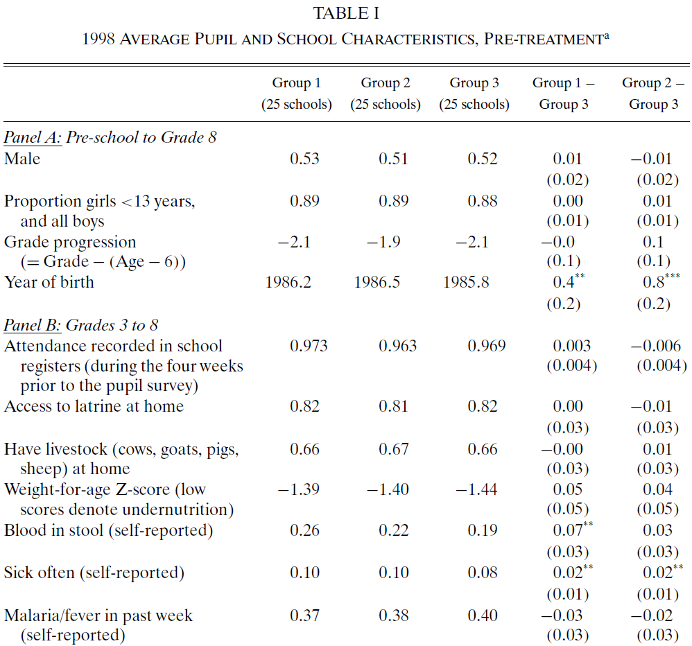
What statistical tools are used to check that control and treatment groups are the same on average?

• Checks and balance tables

  • performs a mean-difference test between treatment and control for

  • variables that are (should be) independent of treatment

• No significant differences (failing to reject \(H_0\)) suggest that the two groups are the same on average

• Any significant differences (rejecting \(H_0\) at the \(\alpha\) level of significance) imply that the two groups are not random.

Ceteris Paribus

Other things are equal! The “other things” are:

• measurable features (age, height, costs, …);

• measurable but absent from our data;

• nonmeasurable factors (ability, effort, connections, …)

Checks and balances table

Source: (Miguel and Kremer 2004) table 1.

Variable-specific means are not the same across groups.

• How to conclude about any difference?

Note: *** indicates p-value < 0.01, ** p-value < 0.05, and * p-value < 0.1.

Hypothesis testing

Formulate \(H_0\) and \(H_1\).

• \(H_0: \text{diff} = 0\)

• \(H_1: \text{diff} \ne 0\)

Use a statistical test, called t-test

• to conclude weather to reject \(H_0\) or fail to reject \(H_0\).

t-tests (1)

Is a statistical test use to conclude about the population based on a sample.

1. One sample t-test: Compares a population parameter \(\mu\) to an arbitrary number?

2. Two sample t-test: Compares difference between two parameters \(\mu_1\) and \(\mu_2\) in the population?

Its purpose is to infer:

• whether or not the population parameter \(\mu\) (mean, or else)

• is different from an arbitrary number (usually zero: \(\mu_{0} = 0\))

• based on our sample estimates of

  • the parameter (\(\widehat{\text{mean}}\)), its variance (\(s\)), and the sample size \(n\).

t-tests (2) Alhorithm 1/2

Step 1: Formulate our Hypotheses

\(H_0: \mu = 0\)

\(H_1: \mu \ne 0\)

Step 2: Compute out Statistics based on the sample

• Estimated parameter: \(\widehat{\mu}\)

• Standard Deviation: \(s\)

• Zero hypothesis value: \(\mu_0 = 0\)

• Significance level: \(\alpha = 0.05\)

• Number of observations: \(n\)

t-tests (3) Alhorithm 2/2

Step 3: Compute t-statistics (and a p-value using the PC)

\[ t = \frac{\hat\mu - \mu_0}{\text{se}} = \frac{\sqrt{n} ( \hat\mu - \mu_0)}{s}\,, \]

where \(se = s / \sqrt{n}\) is the standard error of the estimate;

Step 4: Conclude

1. Reject \(H_0\) if:

   • \(|t| > 2\) the “rule of thumb”

     • The same applies if we say that the estimate is two times larger than the mean.

   • \(\text{p-value} < \alpha\) (probability of type I error < level of significance

2. Fail to reject \(H_0\)

Checks and balances: conclusions

Are the treatment and control groups on average similar?

Table source: (Miguel and Kremer 2004).

Note: *** indicates p-value < 0.01, ** p-value < 0.05, and * p-value < 0.1.

If yes: A mean comparison of the outcome variables reveals the causal effect

If no: We need to use other methods to measure the effect, such as regression.

t-tests (3.1) example

Do the CCTs improve children school enrollment? (Fiszbein et al. 2009)

• The effect: \(\widehat{\text{Enrollment change}} = \widehat{\text{After the CCT}} - \widehat{\text{Before the CCT}}\)

• Hypothesis:

  • \(H_0:\) \(\text{Enrollment change} = 0\)

  • \(H_1:\) \(\text{Enrollment change} > 0\)

• Statistical test:

  • One-sided t-test

  • at the 5% level of significance \(\alpha = 0.05\)

• Desired t-test result:

  • Which t-test result indicates that CCT has a positive effect on school enrollment?

  • \(\text{p-value}\) \(< \alpha\) or \(\text{p-value} < 0.05\)

  • \(|\text{t-statistics}|\) \(> c_{df, \, 0.95}\)

  • We need to be able to reject \(H_0\)

t-tests (3.2) example

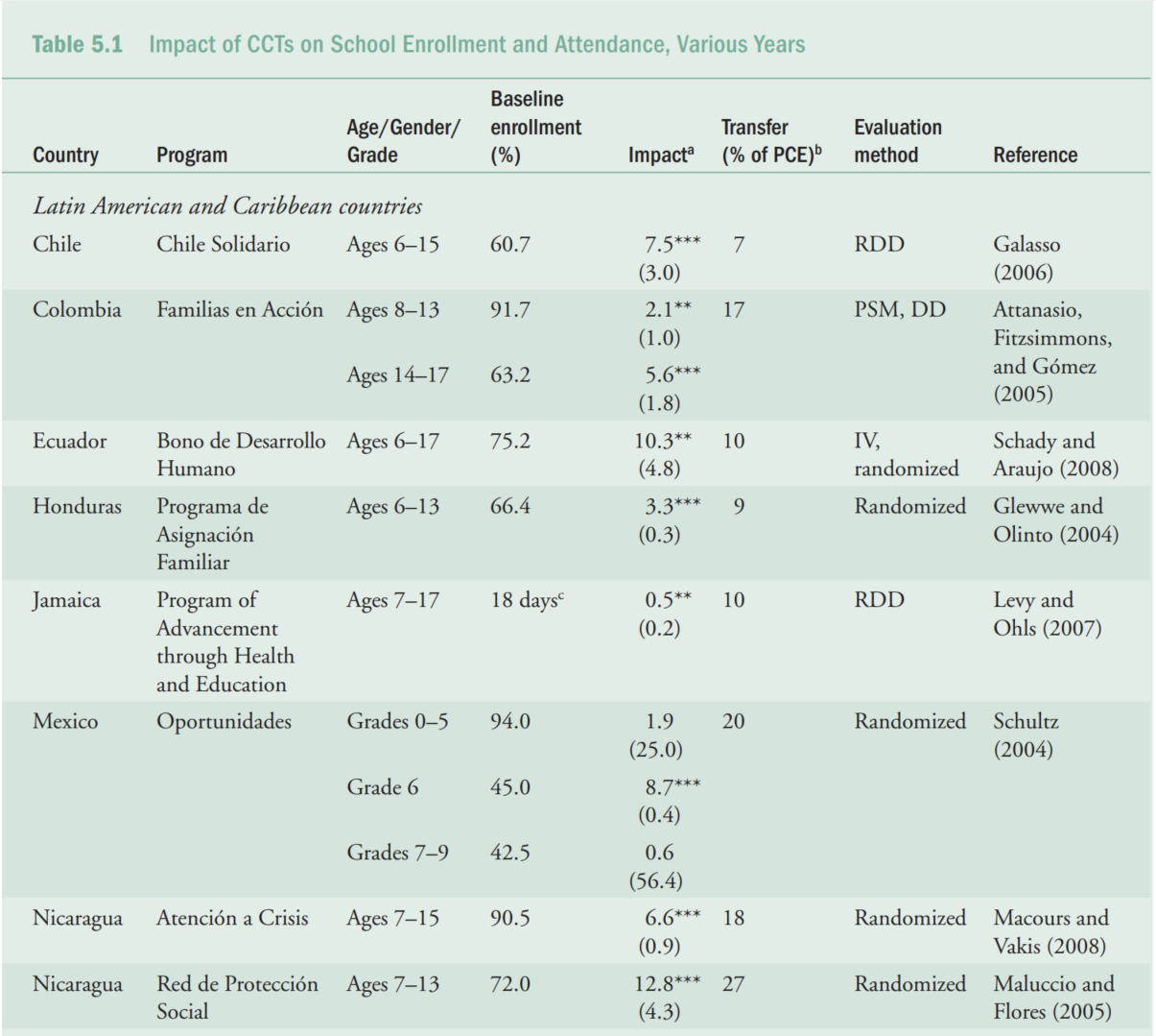
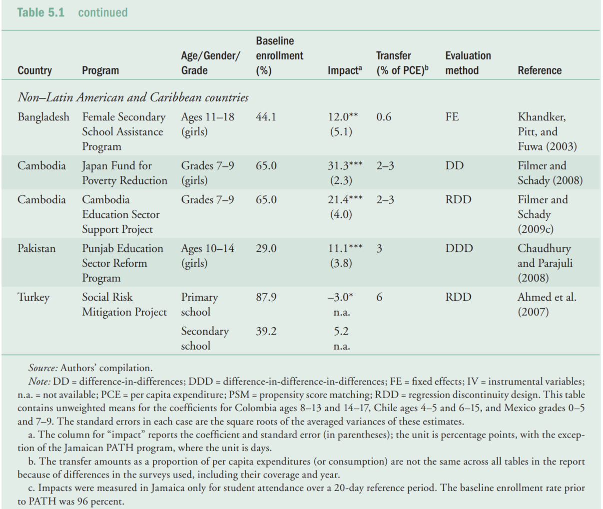
• The column for “impact” reports the difference and standard error (in parentheses); the unit is percentage points, except of the Jamaican PATH program.

• *, **, and *** indicates if the p-value is below a corresponding significance levels of 10, 5, and 1 percent.

• What is shown in the rows?
  • case-specific t-test
• What are \(H_0\) and \(H_1\)?
  • \(H_0: \text{diff} = 0\); \(H_1: \text{diff} \ne 0\);
• What are the conclusions for each row?
  • Reject/Accept \(H_0\)
• What do “stars” imply for test-specific conclusions for each row?

t-tests (3.3) example

Interpret results of the statistical test for country A at the X (1%, 5%) level of significance.

• State Null and Alternative hypotheses.
• Conclude about the HT results.
• What parameter/statistics/number was used to make this conclusion?

For example. In (Ahmed et al. 2007) authors failed to show that CCTs improve/worsen children school enrollment in Turkey. With “H0: no improvement” versus the “H1: some improvement”, the authors failed to reject the H0 at the 5% sign. level for the populations of primary and secondary school attendees …

(For example cont.) … In absolute terms, authors show a reduction in primary school enrollment by 3% and an increase in secondary school enrollment by 5.2%. However, the probability that these changes are due to sample variation (probability of type I error / p-value) is above 5% and 10% respectively. Table source: (Fiszbein et al. 2009)

Homework: Read/do more on Hypothesis testing

OpenIntro Foundations for Inference:

• Point Estimates
• Hypothesis Testing Fundamentals
• Inference for Estimators Other Than the Mean

Khan Academy:

• The idea of significance tests

Normally distributed population and the confidence intervals

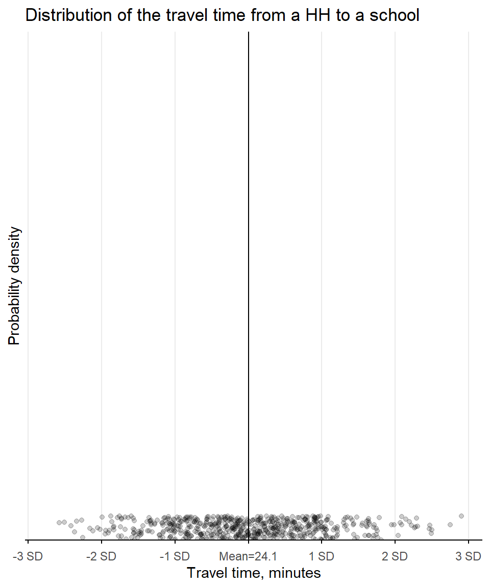
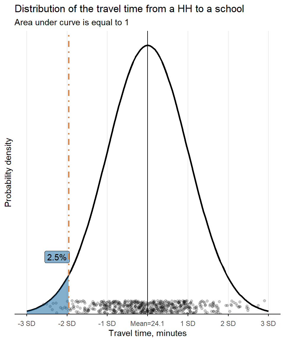
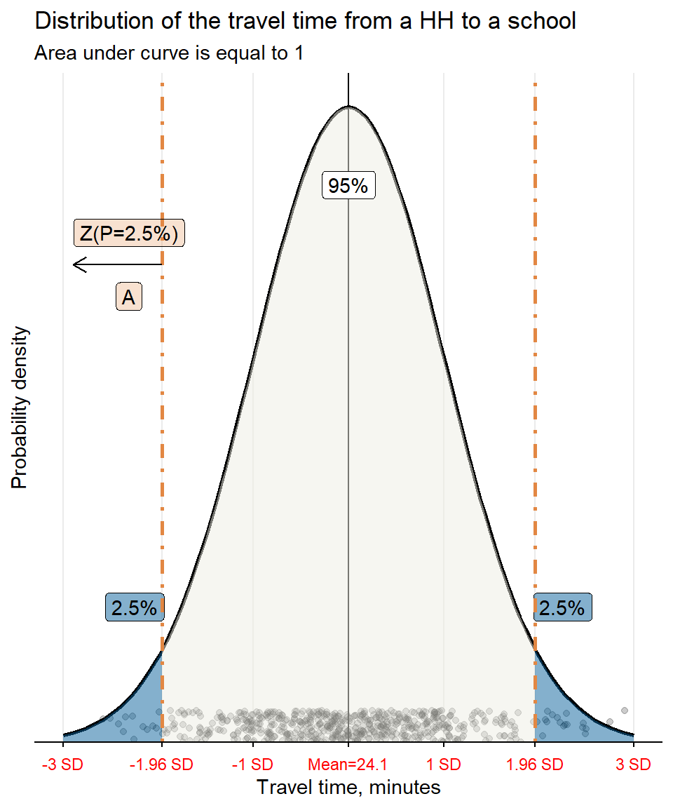
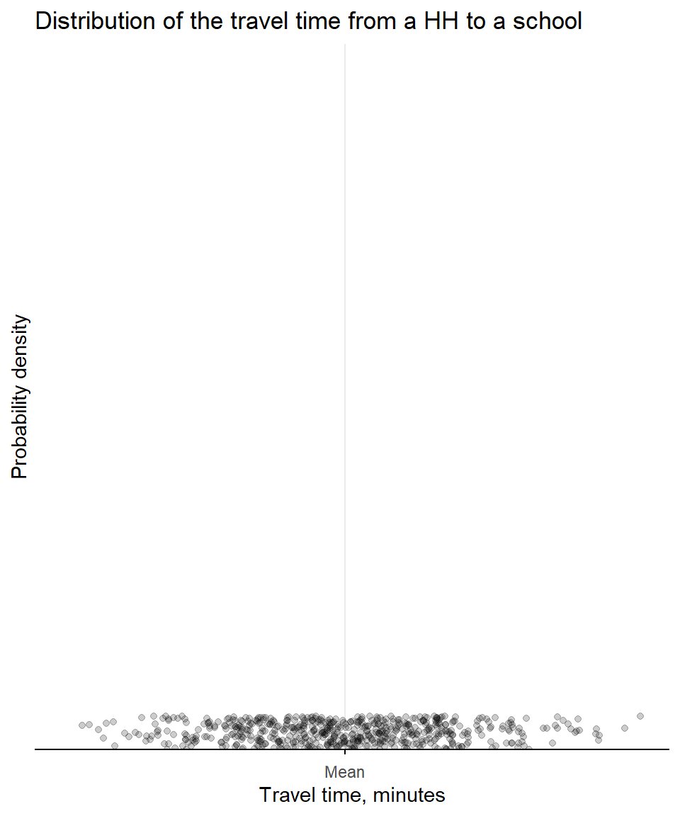
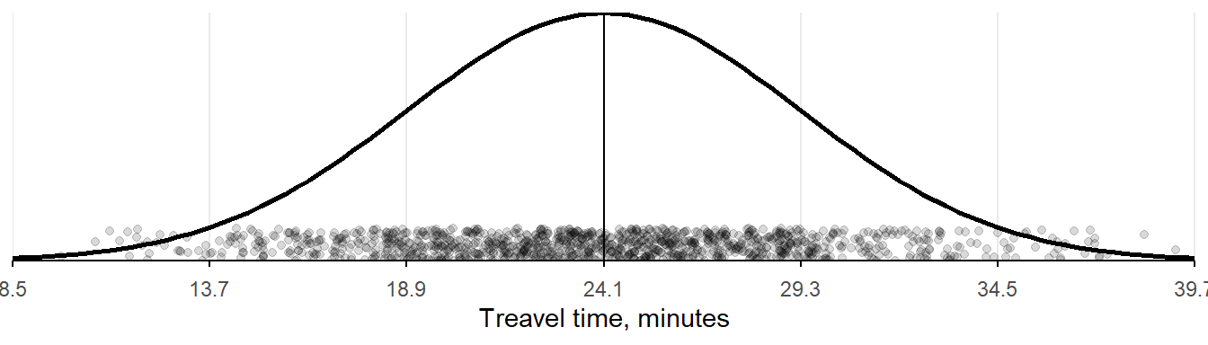
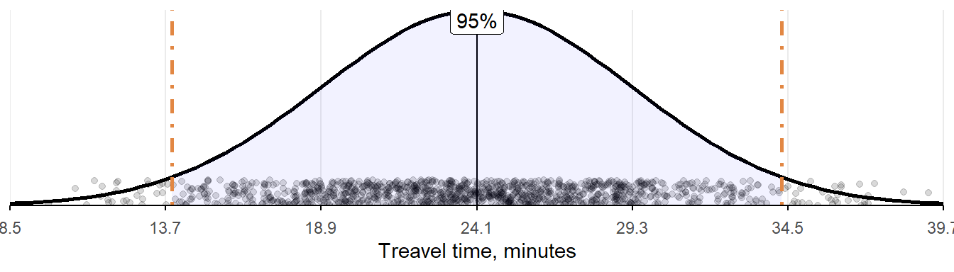
Suppose that we have measured travel time to school for the entire population of the HHs.

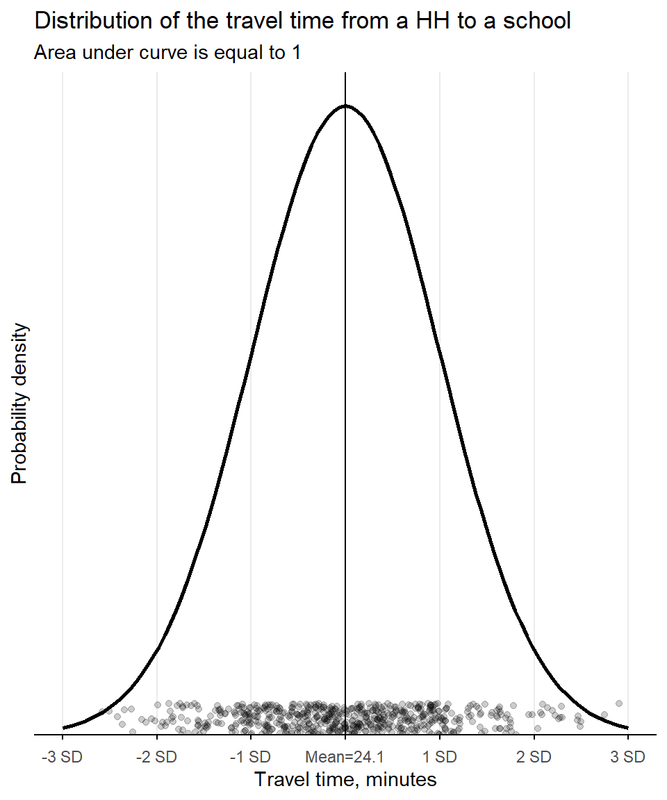
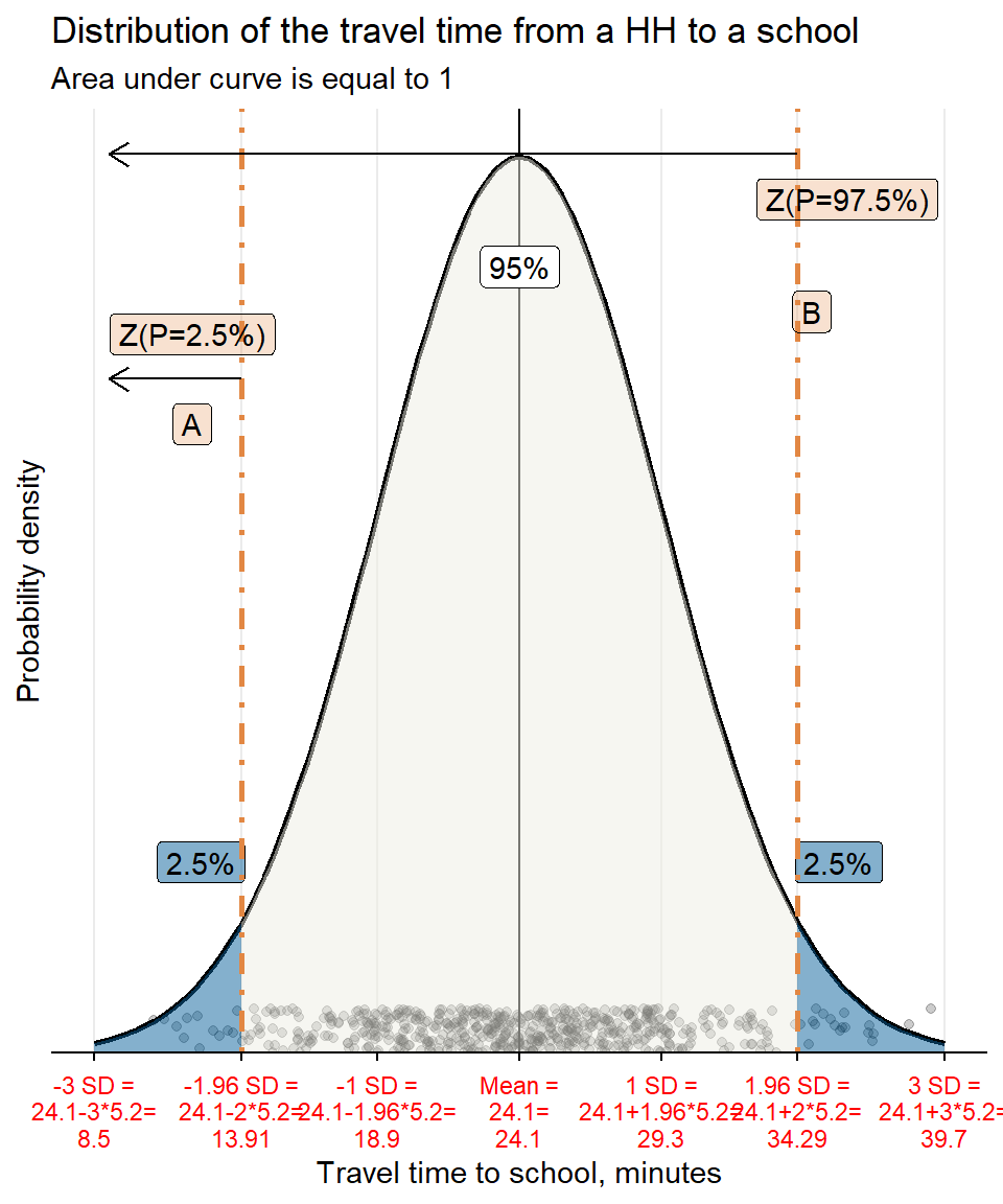
Travel time is distributed normally with:

• \(\mu\) - average travel time;
• \(\sigma\) - standard deviation of \(\mu\);

Population distribution

Travel time distribution is normal with mean \(\mu\) and SD \(\sigma\):

• Within 2 \(\sigma\), there are 95.45% of all observations.

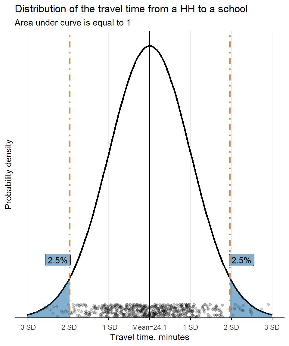
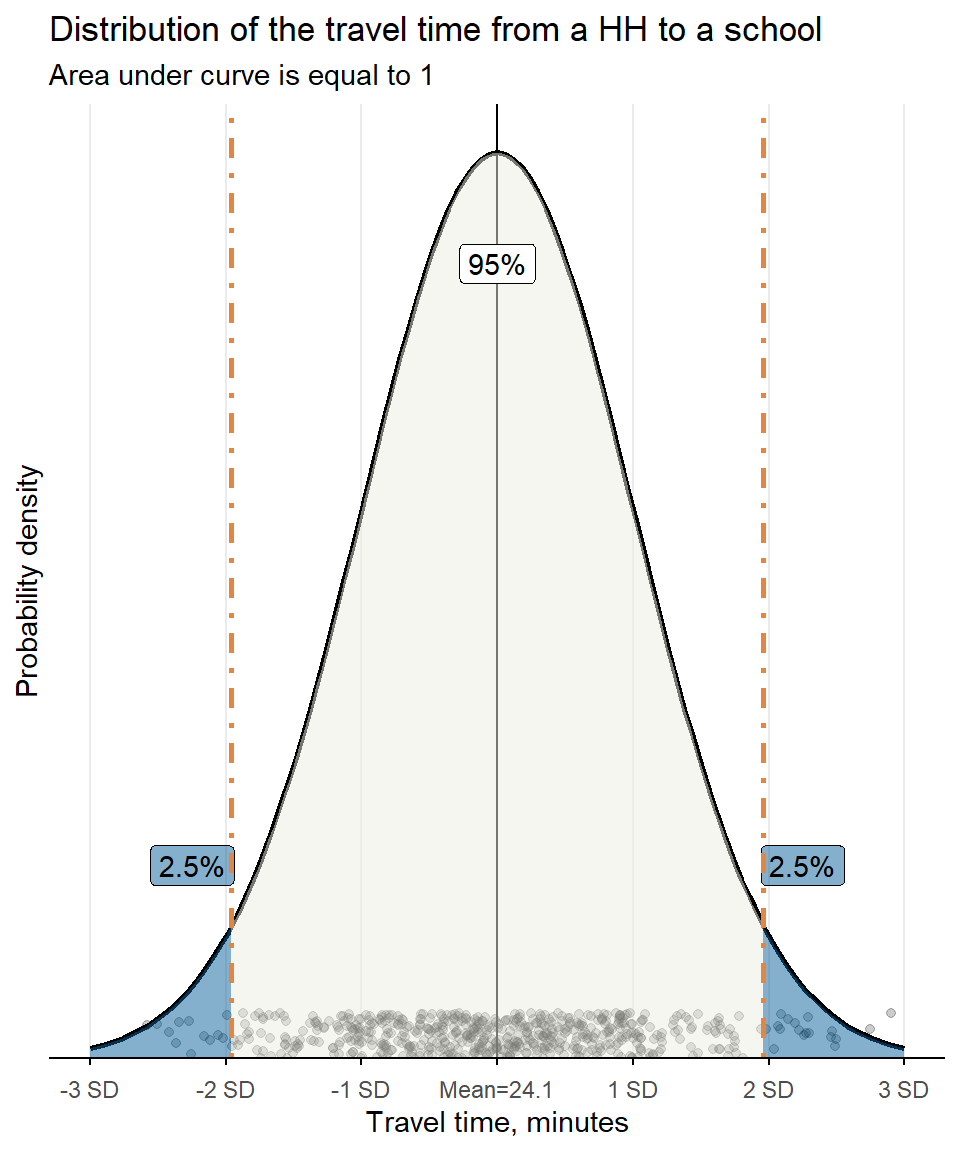
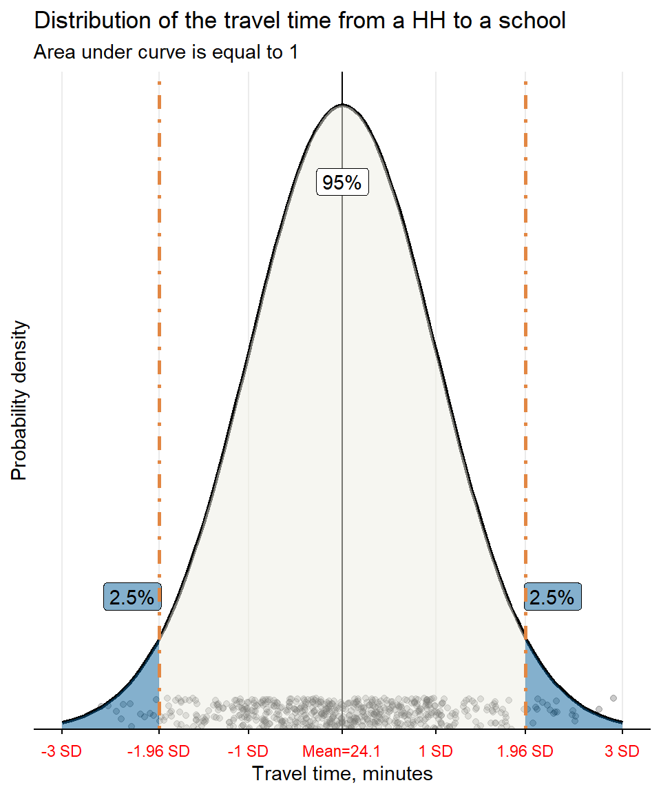
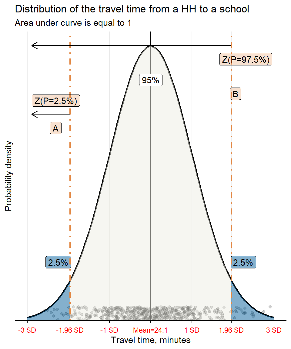
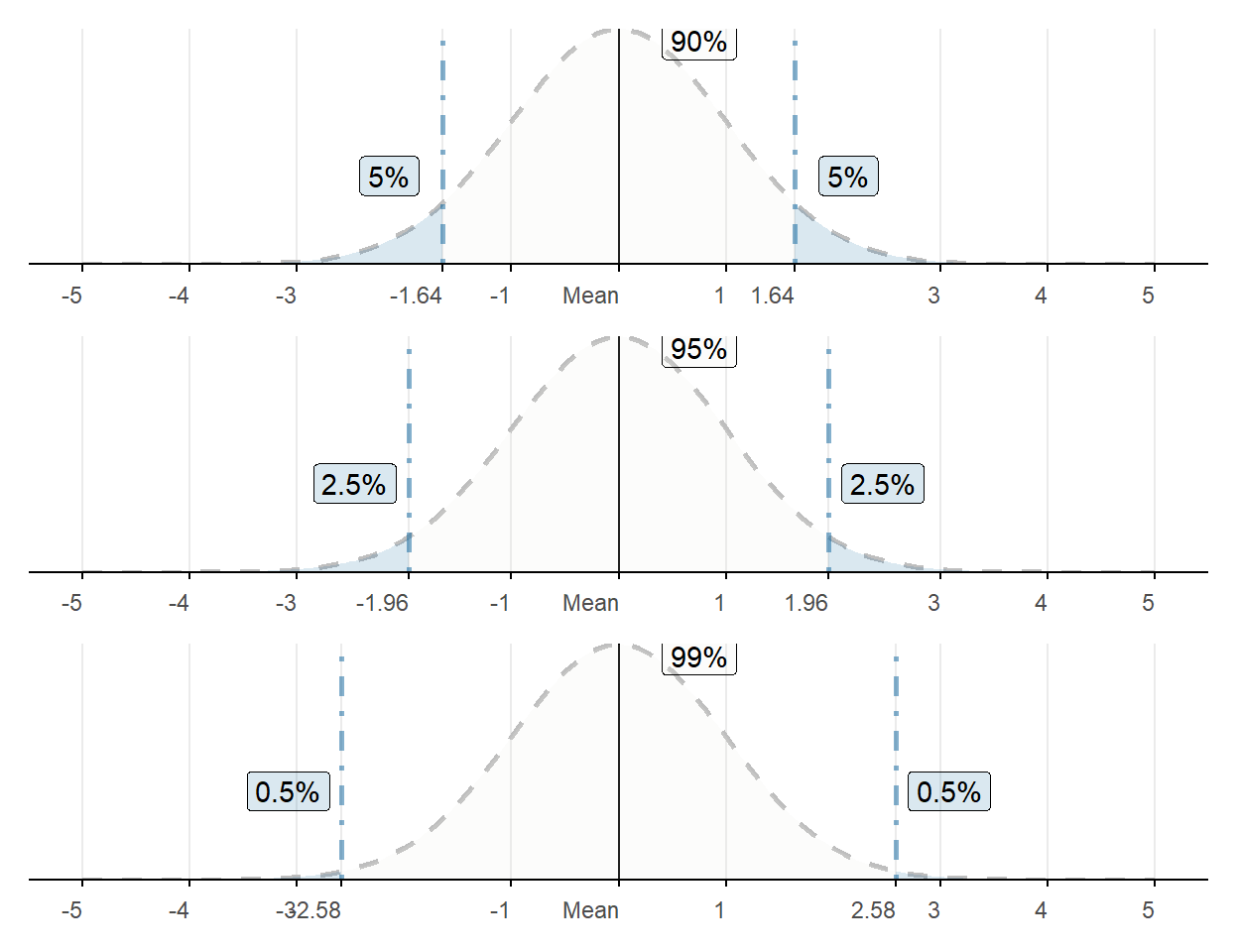
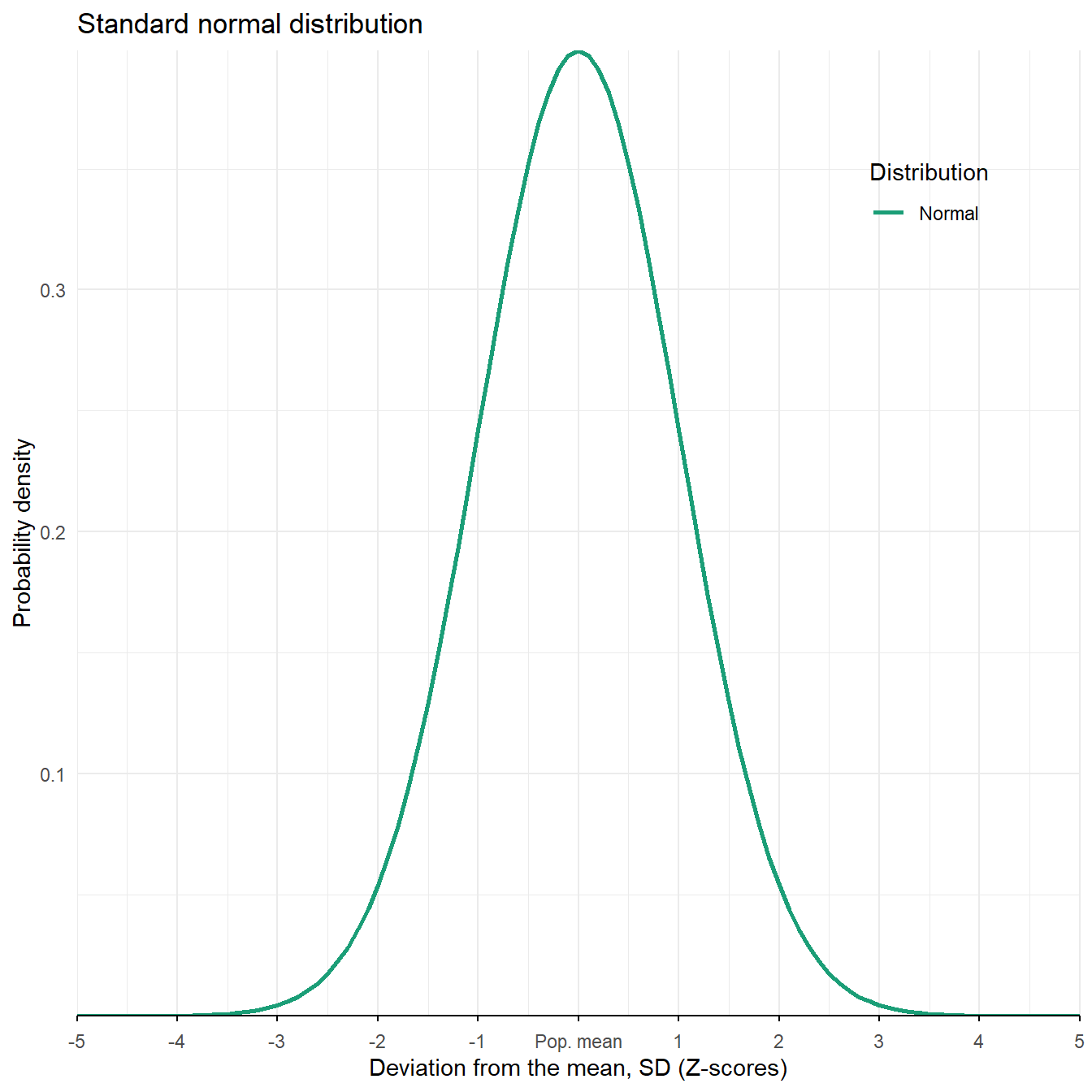
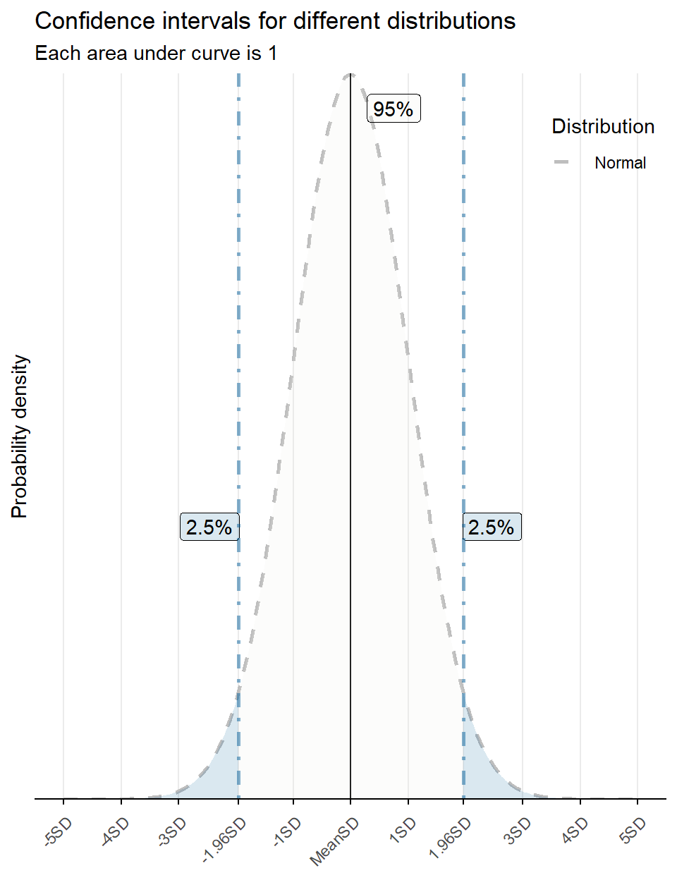
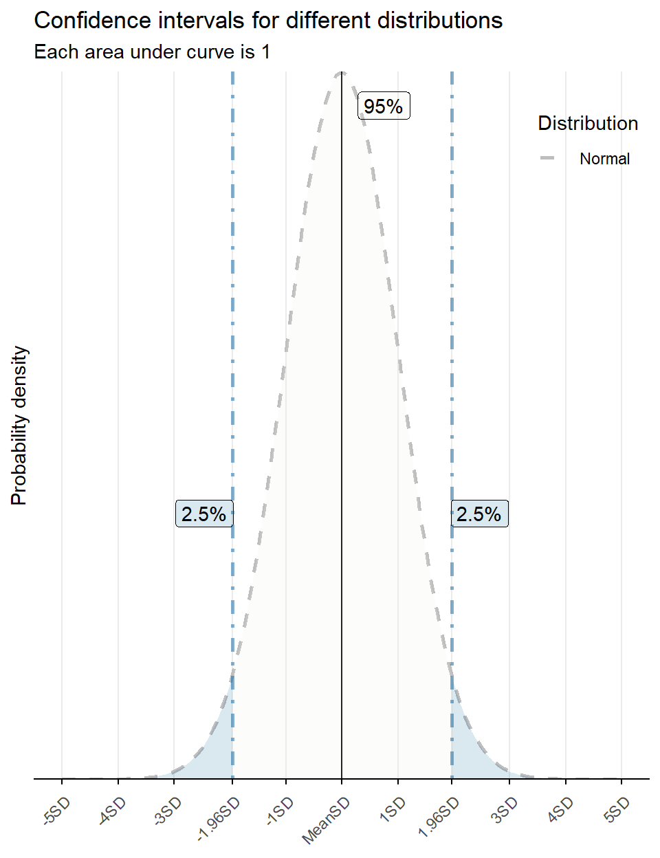
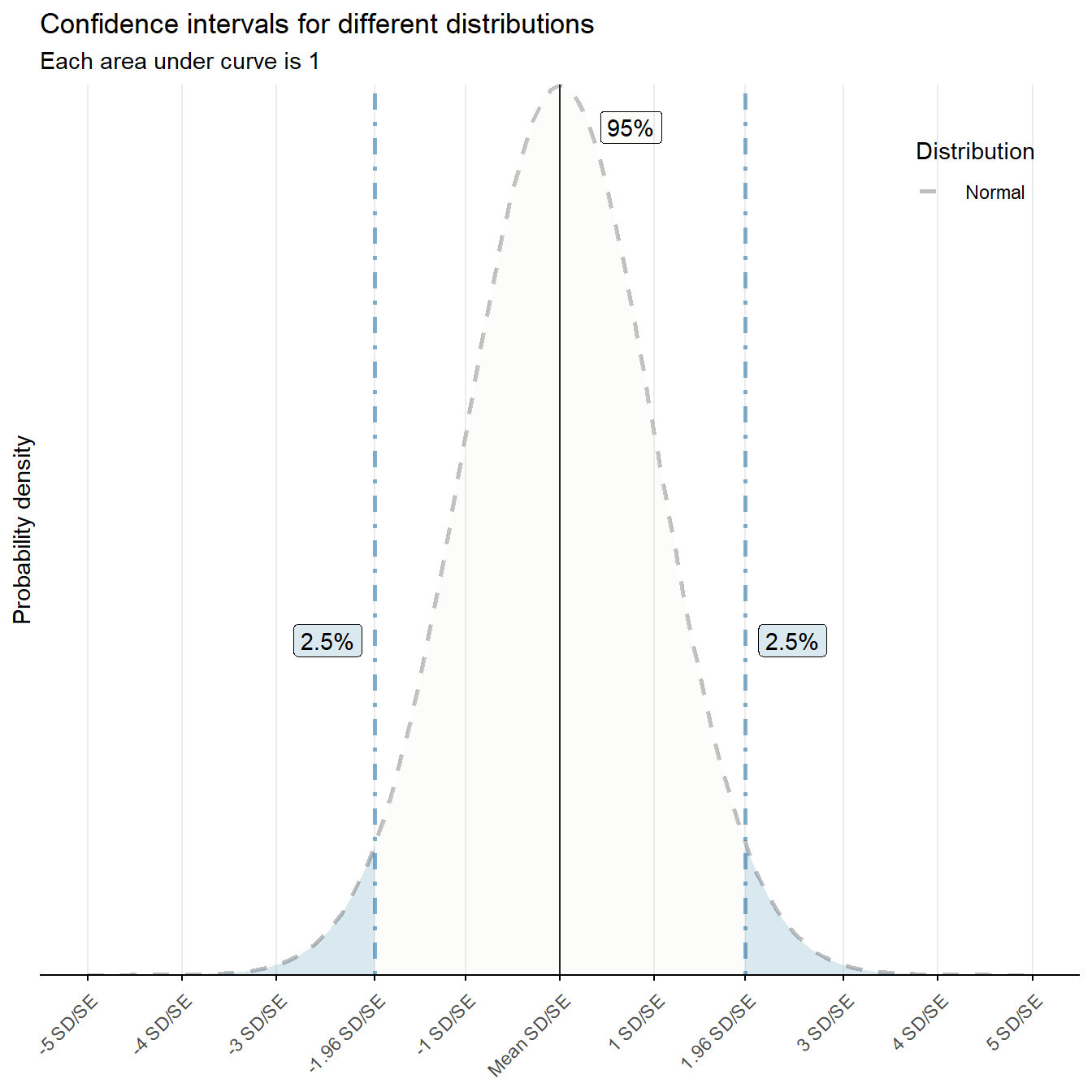
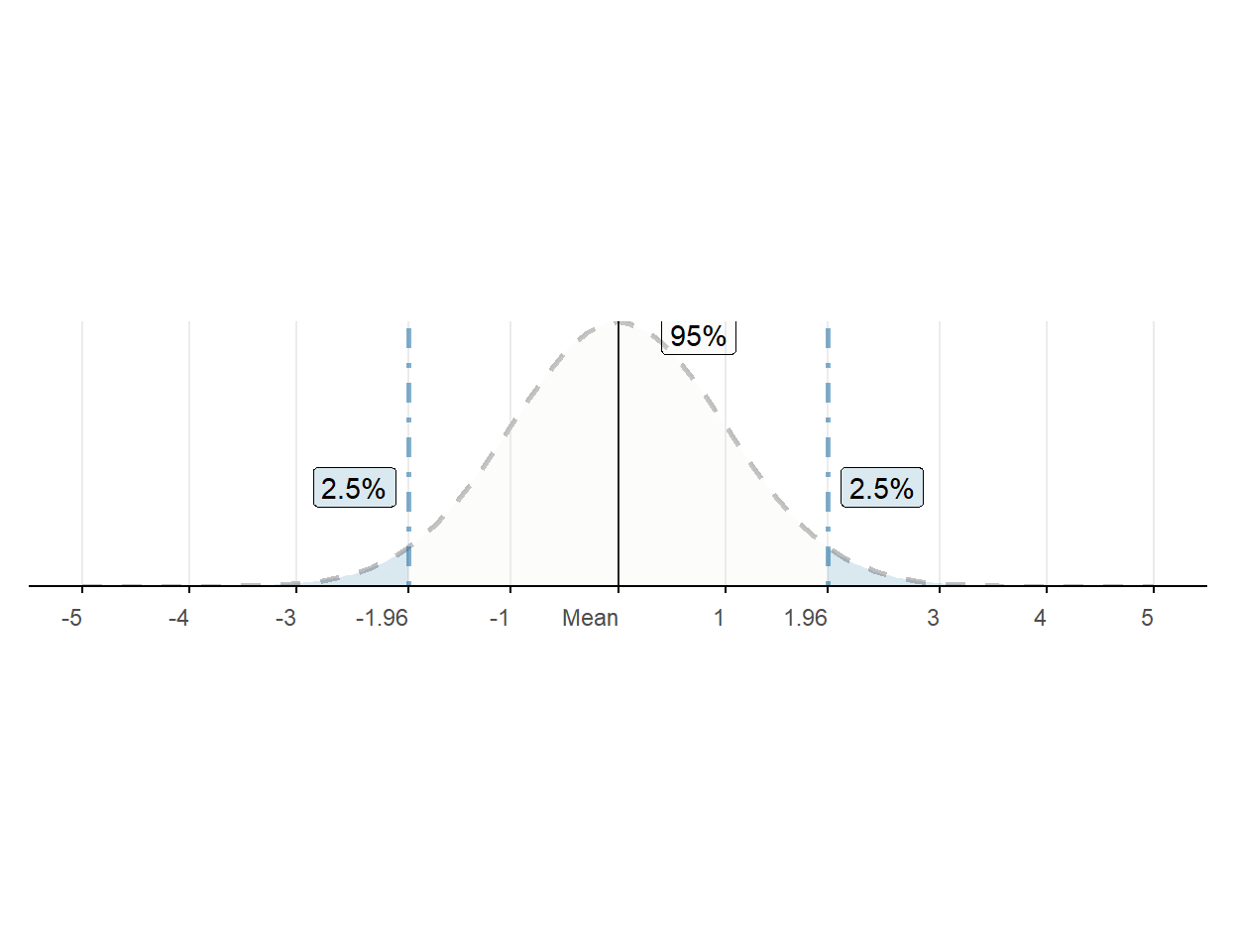
Within what number of \(\sigma\), exactly 95% of all observations are? Any ideas?

95% of HH are located within \(\pm 1.96 \sigma\).

• \(\,1.96 \,\) is the z-score, where:

1. probability to observe travel time below \(\mu - 1.96 \sigma\)

• \(P(x < \mu - 1.96 \sigma) = 0.025\)

2. probability to pick a HH with a travel time below \(\mu + 1.96 \sigma\)

• \(P(x < \mu + 1.96 \sigma) = 0.975\)

95% Confidence interval for the mean is

• an interval (a range), within which we can observe 95% of observations.

• 95% is the confidence level

• 95% confidence level is a convention. Go higher, not lower!

Warning

This definition only applies to the population mean.

Although the idea behind a confidence interval remains the same.

90%, 95% and 99%, Confidence intervals in the population

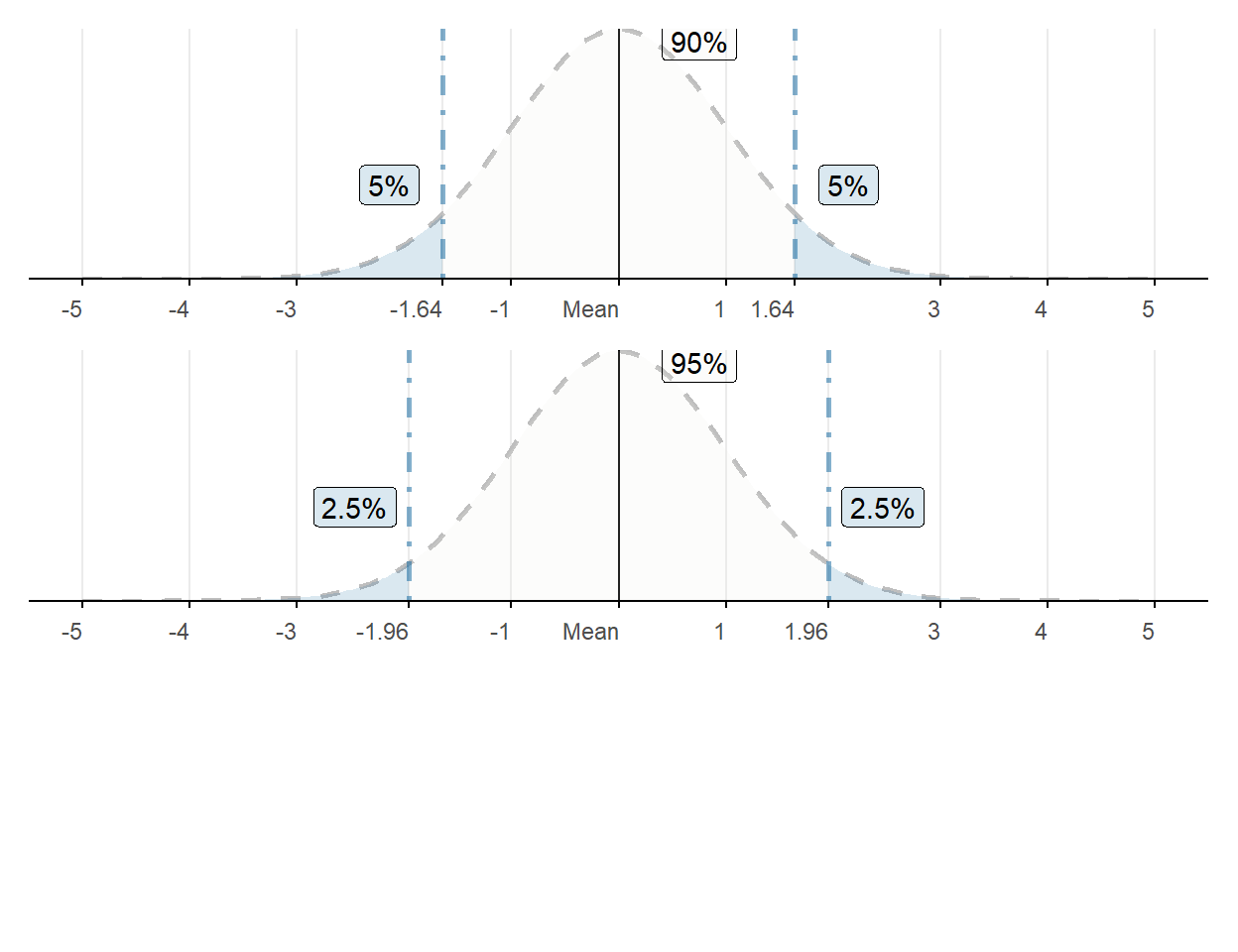
Is 90% confidence interval wider/slimmer than the 95% one?

99% vs 95%?

The population can have any distribution

The Central Limit Theorem (CLT)

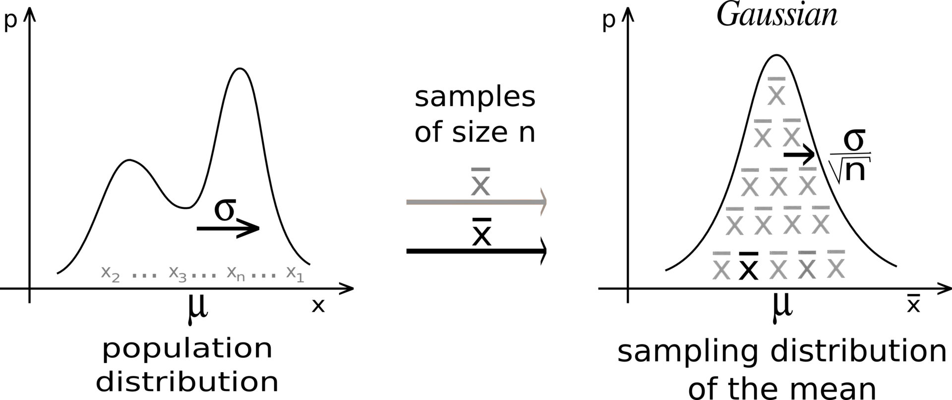
The CLT is the bridge that makes the transition from the population to a sample.

As the sample is used to estimate the population mean, the CLT says that:

• almost any sample average

• is approximately normally distributed,

• with the accuracy of the approximation increasing as the sample size increases (Angrist and Pischke 2014, 39)

The Central Limit Theorem (2)

The estimate of the mean \(\hat{\mu}\) in the sample of the size \(n\)

• tends to follow a normal distribution centered at the population’s mean \(\mu\),

• with the standard error, \(\text{SE}(\hat{\mu})\) calculated based on the population’s standard deviation, \(\text{SE}(\hat{\mu}) = \sigma / \sqrt{n}\),

• when two conditions are satisfied:

  1. Independence. The sample is random.

  2. Only for sample size below 30 obs (\(n < 30\)) Normality. The population is normally distributed.

• See: (Diez et al. 2022)

The Central Limit Theorem (3)

In other words:

• When our random sample is large enough

  • (or the population is normally distributed for small samples),

• sample estimate of mean \(\hat{\mu}\) approximates the population mean \(\mu\):

  • \(\hat{\mu} \approx \mu\);

• with the standard error that depends on the \(\sigma\) (pop. SD) and the sample size (\(n\)):

  • \(\text{SE}(\hat{\mu}) = \sigma / \sqrt{n}\).

The Central Limit Theorem (4)

Because the population’s SD (\(\sigma\)) is unknown, we rely on the sample to estimate:

• the standard error:

  • \(\text{SE}(\hat \mu) = \sigma / \sqrt{n} \approx \hat{\text{SE}}(\hat \mu) = s / \sqrt{n}\),

  • where \(\sigma \approx s\);

• alone with the estimate of mean: \(\hat{\mu} \approx \mu\);

Standard Error (1)

SE is an estimate of the standard deviation in the sampling distribution of \(\hat{\mu}\).

\[\widehat{\text{SE}}(\hat{\mu}) = s / \sqrt{n}\]

Measures deviation (error) of the \(\hat{\mu}\) estimate, from the population parameter (\(\mu\)), accounting for the size of the sample (\(n\)).

Standard Error (2)

“Error” implies that the estimate contains a random error, compared to the population parameter.

• Not to be confused with the Sample Variance

  • \(s^2 = \frac{\sum_{i=1}^N [x_i - \bar{x}]^2 }{N-1}\)

• With the sample size increasing to infinity:

  • standard error approaches to zero,

  • but the sample variance does not!

CLT summary (from <en.wikipedia.org/wiki/Central_limit_theorem>)

CLT in practice

See the following online tools:

• CLT in practics

The Confidence Interval

Supposed that we have a population of unknown distribution, and

• we derive a random sample of a size \(n\) and

• estimate sample mean \(\hat \mu\) and \(\text{SE}(\hat \mu)\)

The Confidence Interval is the range around the sample mean, within which there is a 95% (or 99%) chance of observing our population mean.

How to find a CI?

We need to know:

• how the sample means are distributed,

• when we repeat random sampling from the same population.

The CLT [is very instrumental because it] says:

• sample means are distributed normally, and

• are centered around the population mean,

• when the sample size is large (infinite)

But random samples are finite and often small in size…

The t-distribution

We use t-distribution (instead of the normal) to adjust for the finite sample size and

• to describe the probability distribution of sample mean (\(\hat \mu\)) with variance (\(\text{SE} (\hat \mu)\)).

t-distribution helps us:

• to find the probability that the true population mean is beyond \(\pm \text{SE} (\hat \mu)\) from the \(\hat \mu\), conversely

• tells us how many \(\pm \text{SE} (\hat \mu)\) from the \(\hat \mu\) there is a 95% chance to observe the population mean for the sample of the size \(n\).

From the population to a sample (1)

Sample estimates are less accurate when the size is small.

Therefore, for inference,

• we use t-distribution instead of the normal.

• t-scores instead of the z-scores

t-distribution (1)

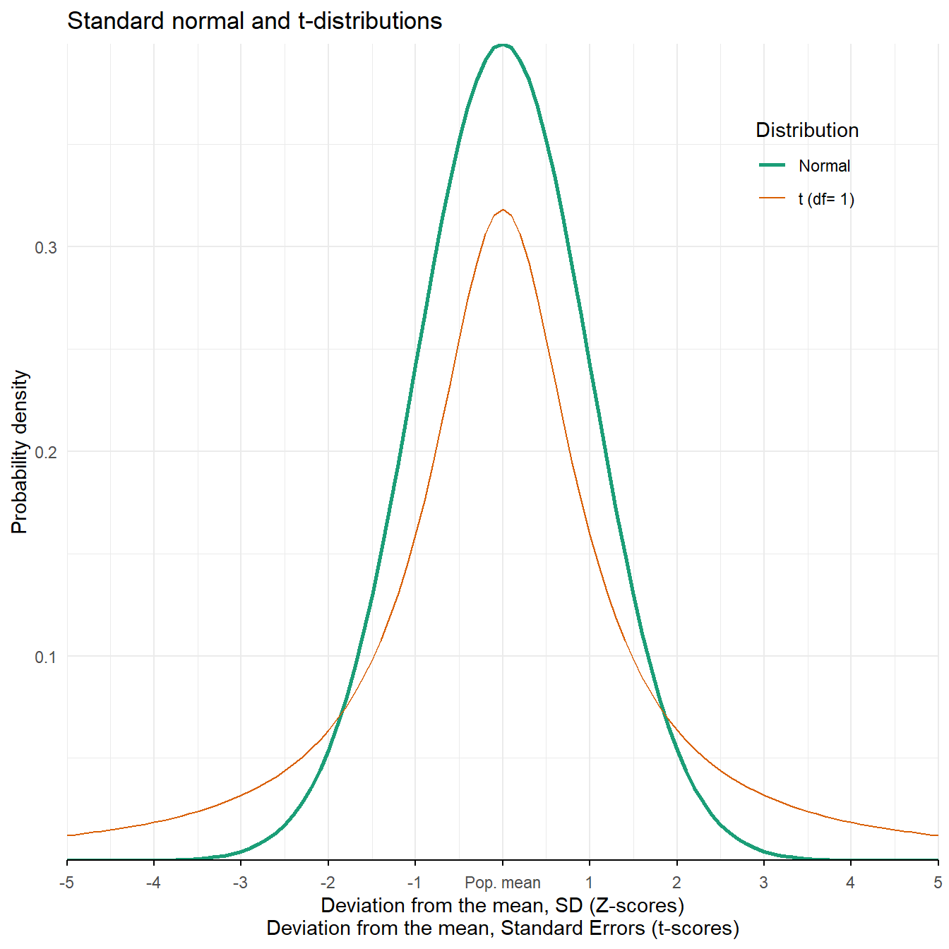
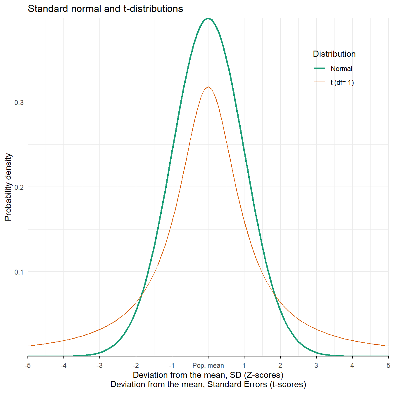
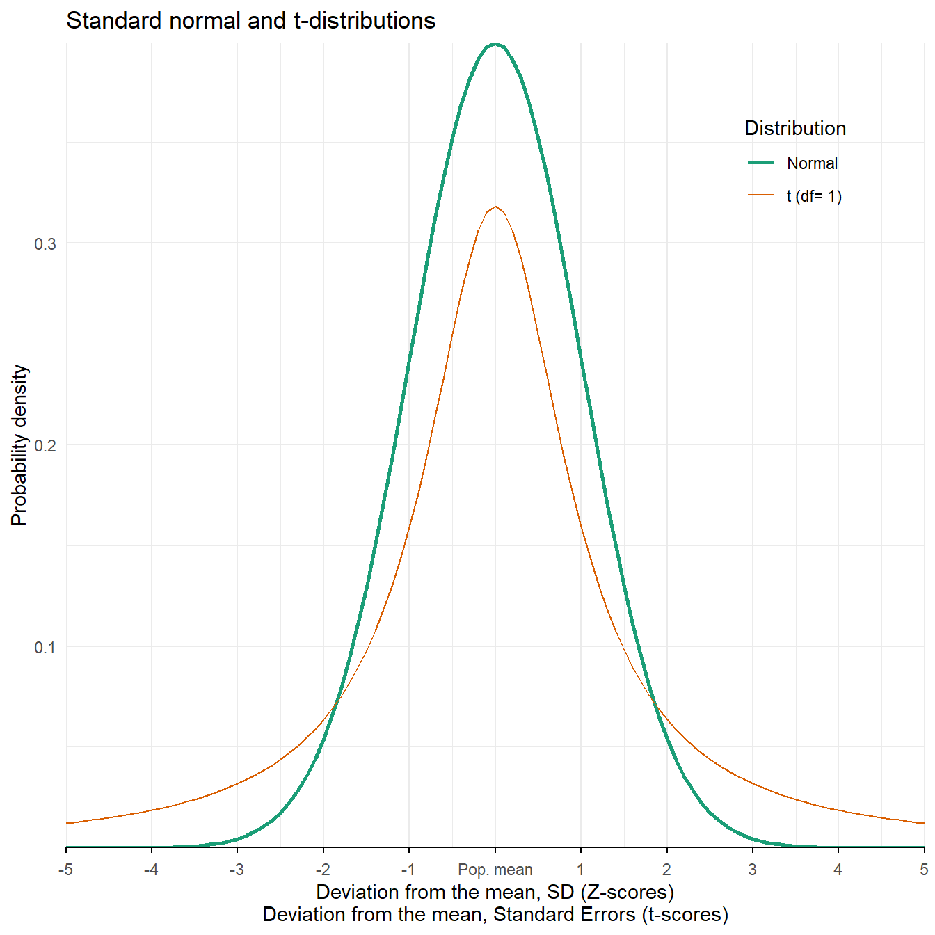
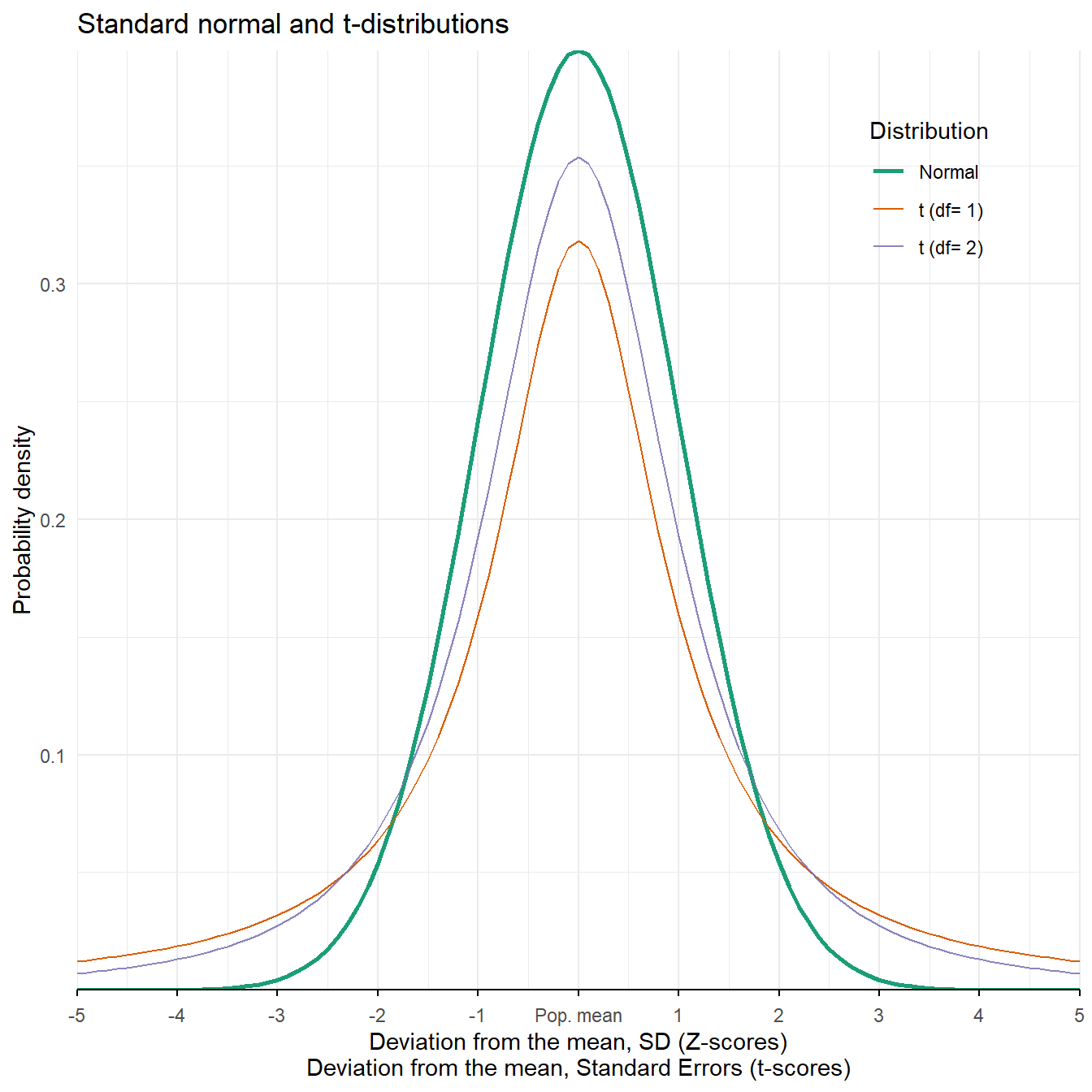
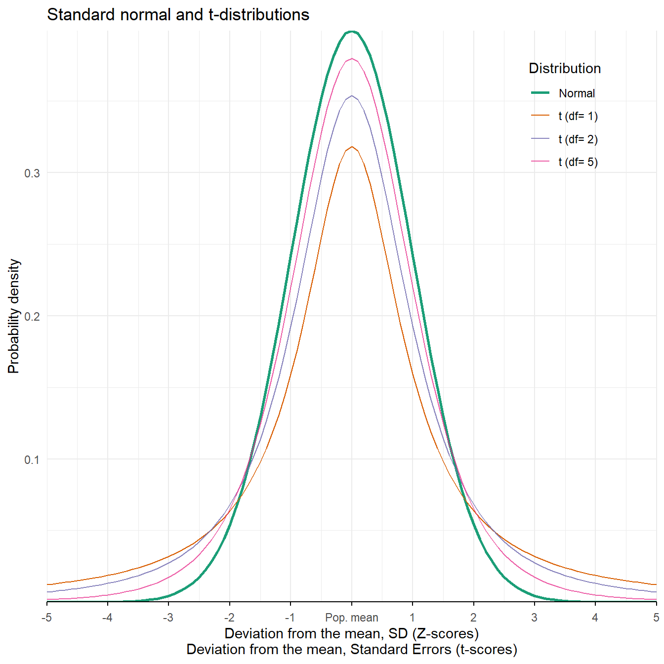
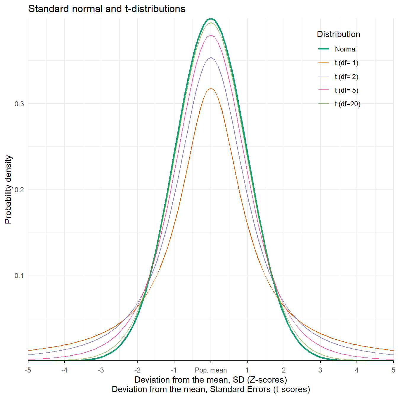
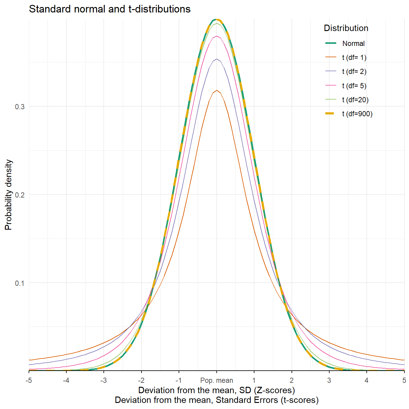
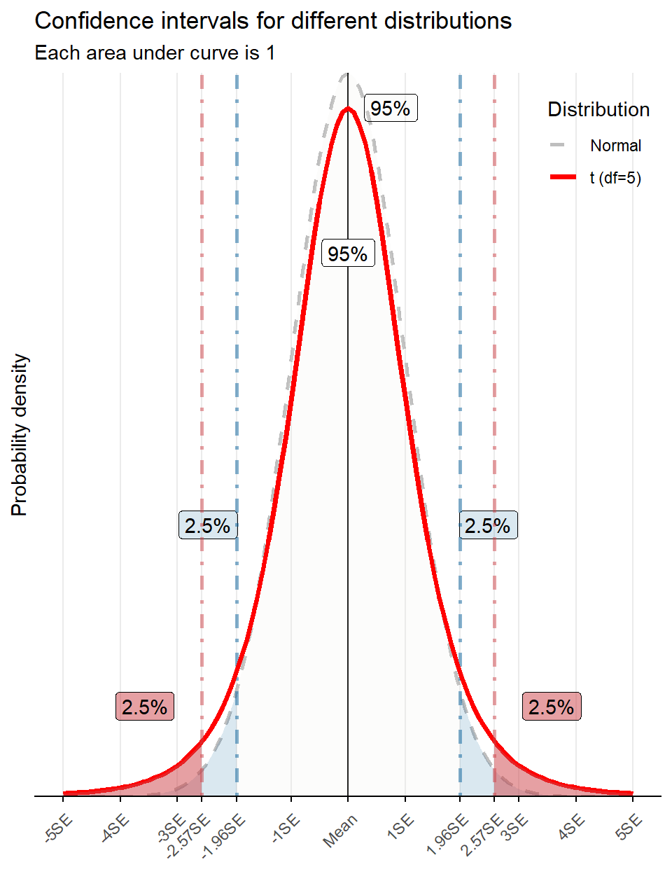
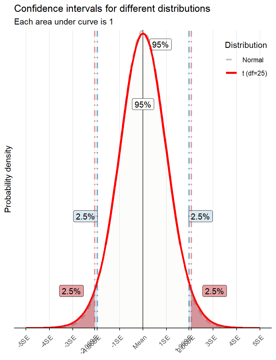
t-distribution has “thicker tails”:

• the probability of observing a more extreme parameter, compared to the population value is larger;

• the peak of t-distribution does not go too high;

• observations are more likely to fall beyond 2SE away from the mean;

t-distribution (2)

The shape of the t-distribution depends on degrees of freedom:

\(df = n - k\), where

\(n\) number of observations in the sample; \(k\) number of estimated parameters;

With an increase in \(df\),

• t-distribution becomes similar to the normal distribution.

t-distribution (3)

Application of the t-distribution

Recall the travel time example

For the population:

• the standard normal distribution and Z-score provide

• the confidence intervals, where we can observe 95% of actual observations.

t-dist in use: travel time (1)

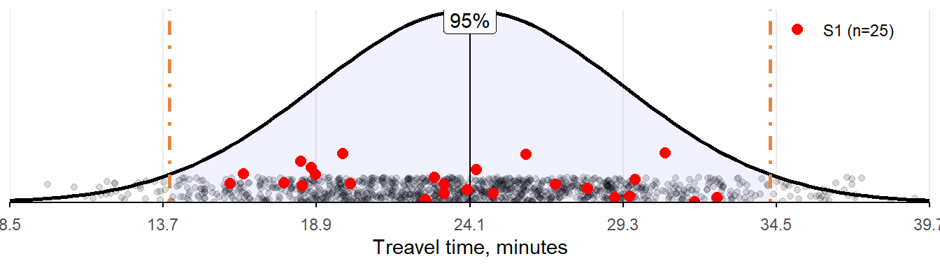
We have a population of travel times to schools.

Let us now:

1 Derive a random sample of N observations.

2 Estimate \(\hat \mu\) and \(\text{SE}(\hat \mu)\)

Sample	\(n\)	\(\hat\mu\)	\(s\)	\(\text{SE}\)
S1	25	23.76	5.04	1.01

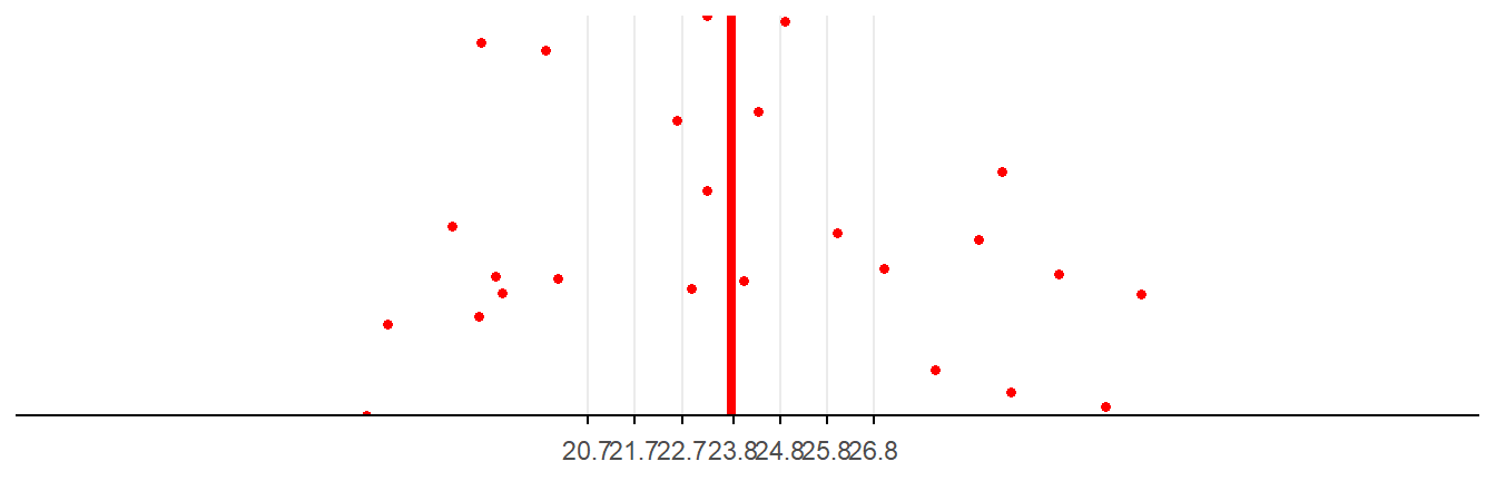
3 Construct the t-distribution for the sample estimates of the mean.

4 Compute 95% confidence intervals: chances that the population mean is within this range are 95%;

5 Conclude that 95% CI is the range where the population mean is 95% likely to be given our sample size, \(\hat \mu\) and \(\text{SE}(\hat \mu)\)

Now, let us repeat steps 1-5 for new samples of different sizes.

t-dist in use: confidence intervals

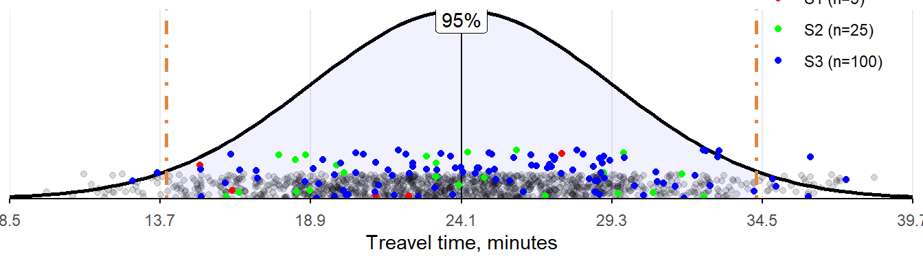
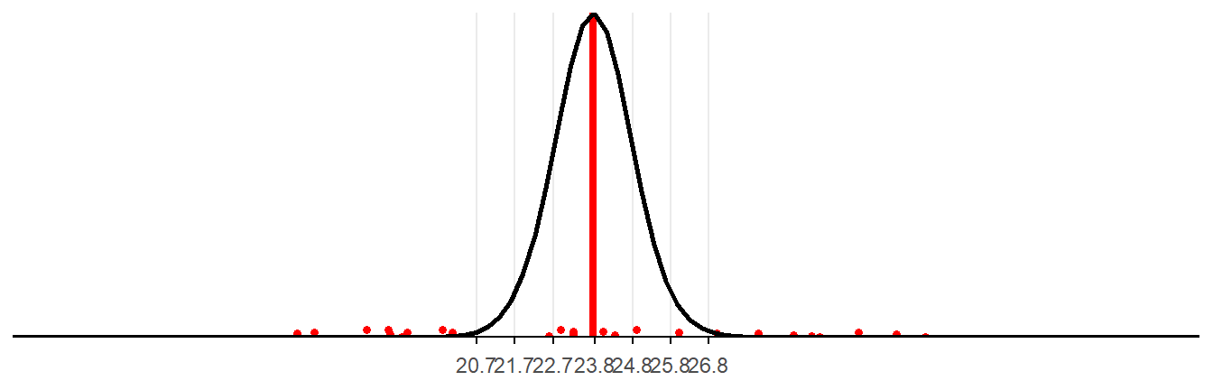
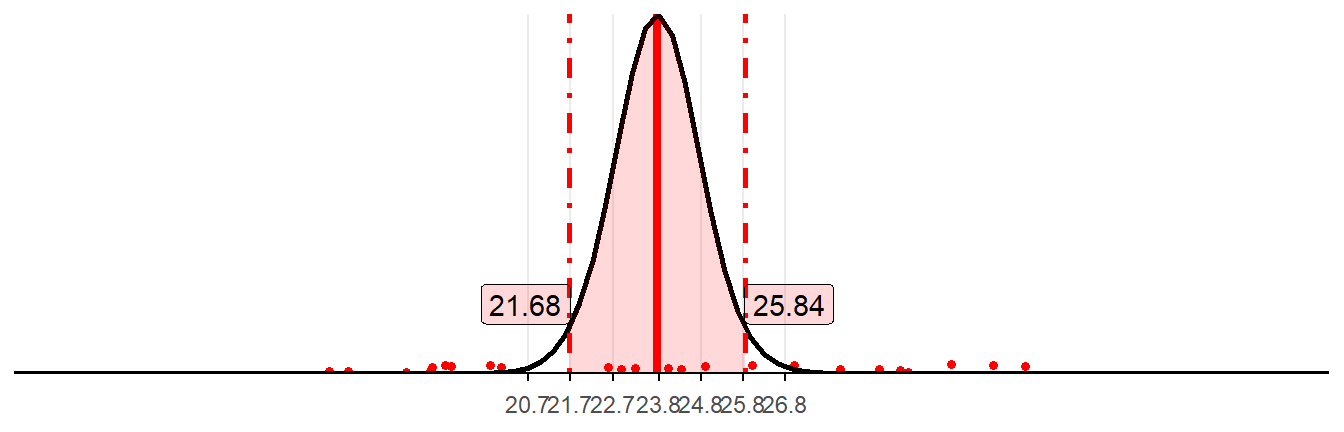
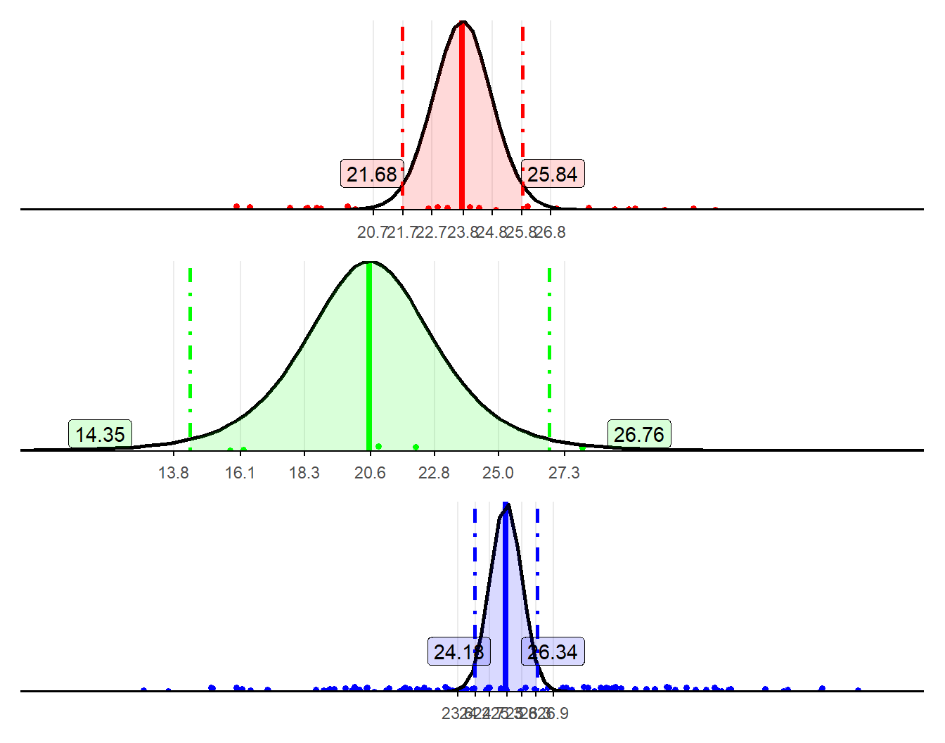
There are four samples of different size:

Each contains estimated parameters, which are different from the population.

Sample	\(n\)	\(\hat\mu\)	\(s\)	\(\text{SE}\)
S1	25	23.76	5.04	1.01
S2	5	20.55	5.00	2.24
S3	100	25.26	5.43	0.54
S4	1000	23.97	5.25	0.17
Pop.	Inf	24.10	5.20	0.00

Using t-distribution, for each sample of size \(n\) we compute a 95% confidence interval.

A 95% confidence interval provides a range, within which the population mean lies with the probability of 95%.

95% Confidence intervals of the mean

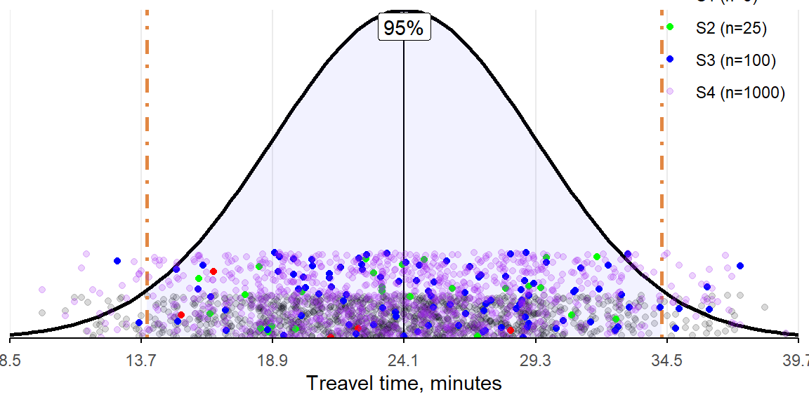
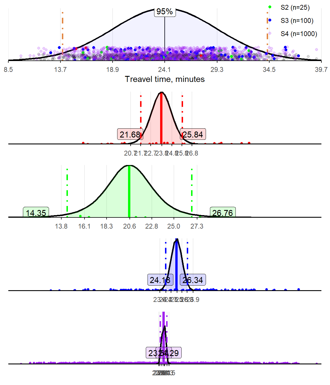
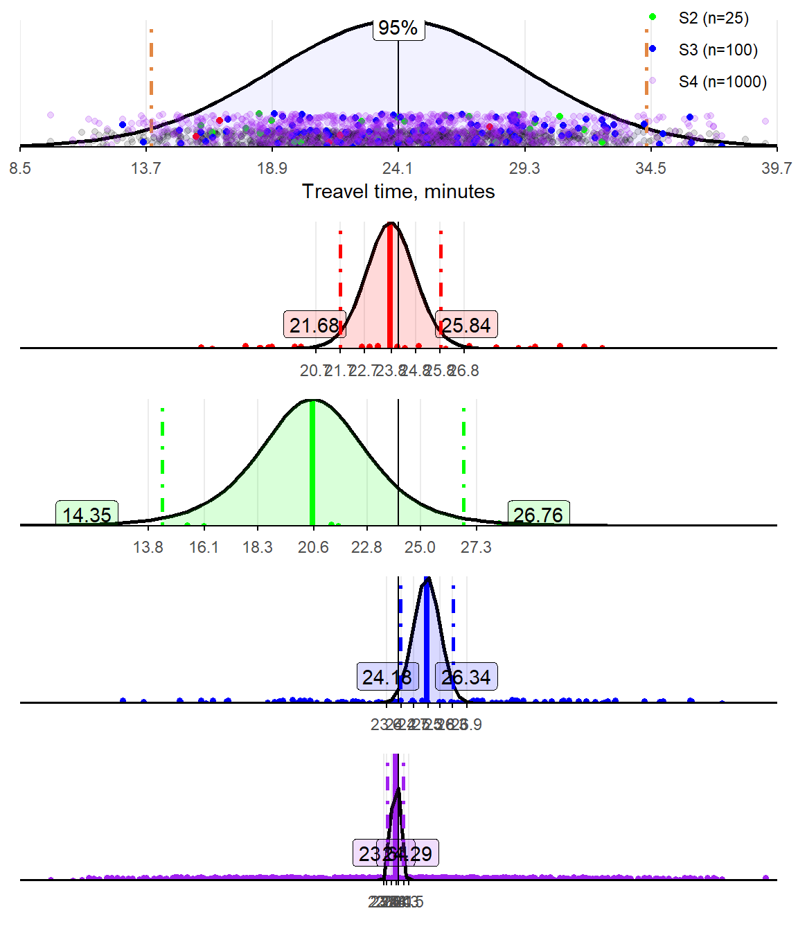
95% confidence interval of the mean is:

• the range, within which we may find the population mean in 95% of random samples made from the same population.

• we are 95% confident in observing the population parameter given the current sample size and \(df\)

90%, 95%, and 99% Confidence intervals of the mean

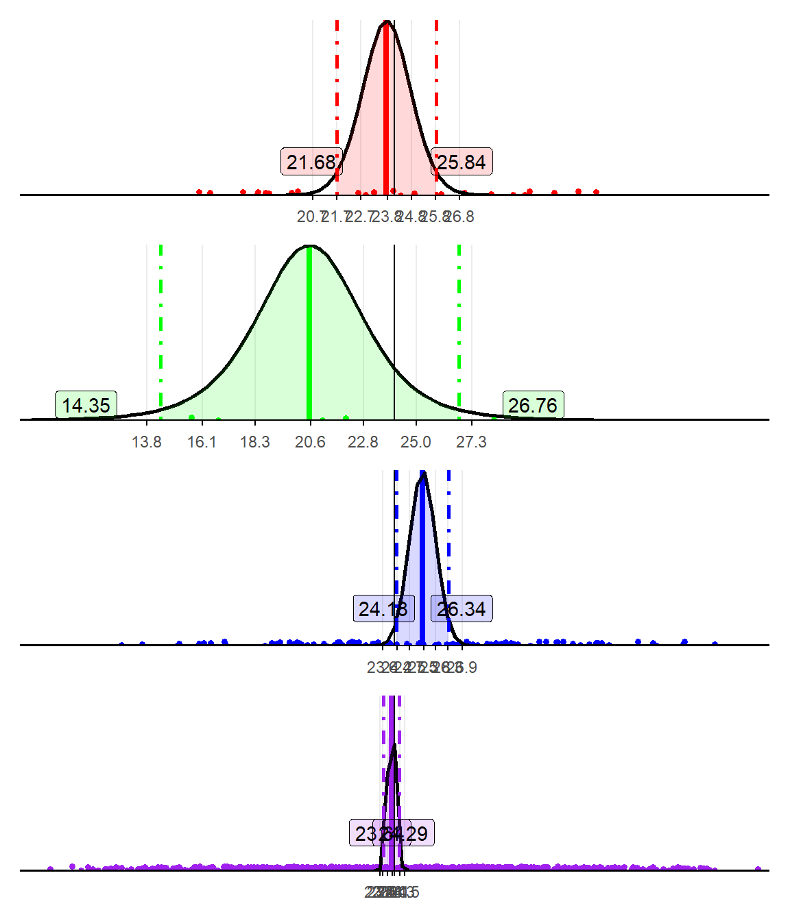
90%, 95%, and 99% are different levels of confidence;

• Confidence level (CL) is the opposite of the level of significance \(\alpha\):

  • \(\text{CL} = 1 - \alpha\)

• It is possible to compute confidence intervals at a different CL.

• They will change in the same way as CI for the normally distributed variable shown before.

Interpreting Confidence Interval

Source: https://rpsychologist.com/d3/ci/

Calculating a Confidence Interval (1)

\(P[...]\) - the probability that the population mean \(\mu\) lies within the lower and upper margins of the confidence interval:

\[P[\hat\mu - c_{df, (1-\alpha/2)} \cdot {\text{SE}}(\hat\mu) \leq \mu \leq \hat\mu + c_{df, (1-\alpha/2)} \cdot {\text{SE}}(\hat\mu) ] = 1 - \alpha\]

• \(\hat\mu\) - estimated mean;
• \({\text{SE}}(\hat\mu)\) - the standard errors;
• \(\alpha\) - level of significance (as before);

• \(\mu\) - unknown population mean;
• \(c_{df, 1-\alpha/2}\) - the critical value of the \(t\) distribution given \(\alpha\), \(df\) and two-tailed test nature;
• \(df\) - number of degrees of freedom (as before);

\[\text{CI} = \{\; \hat\mu - c_{df, (1-\alpha/2)} \cdot {\text{SE}}(\hat\mu)\; ; \; \hat\mu + c_{df, (1-\alpha/2)} \cdot {\text{SE}}(\hat\mu) \; \}\]

Calculating a Confidence Interval (2)

Sample of the size 5 is derived from the population. Estimated statistics for the travel time from HHs to school in minutes are:

Sample	\(n\)	\(\hat\mu\)	\(s\)	\(\text{SE}\)
S2	5	20.55	5	2.24

Calculate the 95 confidence intervals for this mean.

\(df\) is: 4

\(c_{df, (1-\alpha/2)}\) is: \(c_{4, (1-0.05/2)} = 2.776\)

Lower bound is: \(20.55 - 2.24 * 2.776 = 14.331\)

Upper bound is: \(20.55 + 2.24 * 2.776 = 26.769\)

CI is: \([14.331 \; ; \; 26.769]\)

df	0.9	0.95	0.975
1	3.0777	6.3138	12.7062
2	1.8856	2.9200	4.3027
3	1.6377	2.3534	3.1824
4	1.5332	2.1318	2.7764
5	1.4759	2.0150	2.5706
6	1.4398	1.9432	2.4469
7	1.4149	1.8946	2.3646
8	1.3968	1.8595	2.3060
9	1.3830	1.8331	2.2622
15	1.3406	1.7531	2.1314
20	1.3253	1.7247	2.0860
25	1.3163	1.7081	2.0595
50	1.2987	1.6759	2.0086
100	1.2901	1.6602	1.9840
1000	1.2824	1.6464	1.9623

Calculating a Confidence Interval (3)

Sample of the size 25 is derived from the population. Variable measured travel time from HHs to school in minutes. Estimated statistics are:

Sample	\(n\)	\(\hat\mu\)	\(s\)	\(\text{SE}\)
S1	25	23.76	5.04	1.01

Calculate the 99 confidence intervals for this mean.

\(df\) is: 4 \(c_{4, (1-0.01/2)}\) is: 2.064

Lower bound is: \(23.76 - 1.01 * 2.064 = 21.675\)

Upper bound is: \(23.76 + 1.01 * 2.064 = 25.845\)

CI is: \(21.675 \; ; \; 25.845\)

df	0.975	0.99	0.995
1	12.7062	31.8205	63.6567
2	4.3027	6.9646	9.9248
3	3.1824	4.5407	5.8409
4	2.7764	3.7469	4.6041
5	2.5706	3.3649	4.0321
6	2.4469	3.1427	3.7074
7	2.3646	2.9980	3.4995
8	2.3060	2.8965	3.3554
9	2.2622	2.8214	3.2498
15	2.1314	2.6025	2.9467
20	2.0860	2.5280	2.8453
25	2.0595	2.4851	2.7874
50	2.0086	2.4033	2.6778
100	1.9840	2.3642	2.6259
1000	1.9623	2.3301	2.5808

More on the t-distribution and t-test

Open intro:

7.1A - t-distribution

7.1B - Inference for one mean

7.2 - Paired data

7.3 - Difference of two means

Khan academy:

Module: Tests about a population mean

More significance testing videos

Practice

Example 1: Effect of a drug on sleep (1)

Question: Does the drug increase sleeping time at the 5% level of significance?

• Null hypothesis: the drug has a zero effect
• Alternative: the drug has a nonzero effect

Data:

• sleep time for each patient before they started taking drugs (control)
• the same after they took drugs (treatment)
• for each patient separately, we computed a difference in sleep time between control and treatment.
• measures are made for 10 patients

The estimated parameters are:

vars	n	mean	sd	se
1	10	0.75	1.78901	0.5657345

• Can we conclude that the mean is different from zero?

Example 1: Effect of a drug on sleep (2)

Can we conclude that the mean is different from zero?

• NO! we cannot.

Because:

• the mean difference could result from a small sample or sample’s variation.

• to conclude about the population, we need to take into account the sample distribution.

We need to perform a Statistical Hypothesis Testing with:

• The one-sample two-sided t-test.

• Compare mean to a zero;

One-sample t-test (1): What?

One-sample t-test

• \(H_0\) mean is equal to the parameter mu specified (or zero if not specified);

• \(H_1\) mean is not equal to zero;

• To decide whether to reject or accept the null hypothesis, we need to rely on:

t.test(slp$extra, mu = 0)
#   One Sample t-test
# data:  slp$extra
# t = 1.3257, df = 9, p-value = 0.2176
# alternative hypothesis: true mean is not equal to 0
# 95 percent confidence interval:
#  -0.5297804  2.0297804
# sample estimates:
# mean of x 
#      0.75 

• The test of significance
• The confidence interval
• The p-value

One-sample t-test (2): The Test of Significance

1. Check the \(t\) statistics against the critical value \(c_{df , \, 1 - \alpha / 2}\).

t.test(slp$extra, mu = 0)
#   One Sample t-test
# data:  slp$extra
# t = 1.3257, df = 9, p-value = 0.2176
# alternative hypothesis: true mean is not equal to 0
# 95 percent confidence interval:
#  -0.5297804  2.0297804
# sample estimates:
# mean of x 
#      0.75 

• \(df=9\)
• \(c_{0.975, 9} = 2.2622\)
• if \(|t| \leq c_{df , \, 1 - \alpha / 2}\) - fail to reject \(H_0\);

• if \(|t| > c_{df , \, 1 - \alpha / 2}\) - reject \(H_0\) in favor of \(H_1\) at \(\alpha\) significance level;

One-sample t-test (2): Confidence intervals

2. Check the confidence interval of the mean

t.test(slp$extra, mu = 0)
#   One Sample t-test
# data:  slp$extra
# t = 1.3257, df = 9, p-value = 0.2176
# alternative hypothesis: true mean is not equal to 0
# 95 percent confidence interval:
#  -0.5297804  2.0297804
# sample estimates:
# mean of x 
#      0.75 

• if CI includes the value from \(H_0\) (0) - fail to reject \(H_0\);

• if CI does not include the number from \(H_0\), we reject \(H_0\) in favor of \(H_1\) at \(\alpha\) significance level;

One-sample t-test (2): p-value

t.test(slp$extra, mu = 0)
#   One Sample t-test
# data:  slp$extra
# t = 1.3257, df = 9, p-value = 0.2176
# alternative hypothesis: true mean is not equal to 0
# 95 percent confidence interval:
#  -0.5297804  2.0297804
# sample estimates:
# mean of x 
#      0.75 

• if \(p-value < \alpha\), we reject \(H_0\) in favor of \(H_1\) at the \(p-value\) significance level;

• if \(p-value \geq \alpha\), we fail to reject \(H_0\);

One-sample t-test (3): Conclusion

t.test(slp$extra, mu = 0)
#   One Sample t-test
# data:  slp$extra
# t = 1.3257, df = 9, p-value = 0.2176
# alternative hypothesis: true mean is not equal to 0
# 95 percent confidence interval:
#  -0.5297804  2.0297804
# sample estimates:
# mean of x 
#      0.75 

• We fail to reject \(H_0\)

• The evidence is insufficient to conclude that the change in sleep time is significantly different from 0 at the 5% level of the sign.

Example 2: Travel time difference between treatment and control

We come back to the travel time example.

Checks and balances

Travel time example:

• Two random samples are derived from the population:

  • Treatment, where (CCTs) were provided;

  • Control, where no CCT was provided;

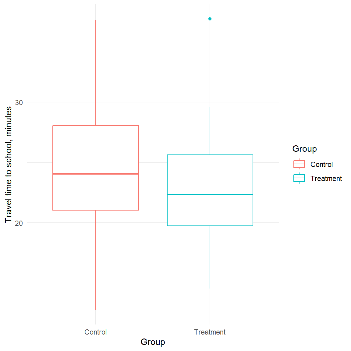
We want to establish that the mean travel times of these two groups are similar on average.

Exploratory analysis (1)

From the plot, we observe:

1. Medians are slightly different but they overlap within the boxes (for 50% of all observations)

2. Variances are different based on the whiskers. The presence of an outlier in the treatment may indicate that groups have similar variances, but the small sample size does not perfectly represent it.

3. We may consider using a t-test for two samples with unequal variances.

Exploratory analysis (2)

Group	\(n\)	\(\hat\mu\)	\(s\)	\(\text{SE}\)
Control	31	24.46	5.52	0.99
Treatment	33	23.01	4.64	0.81

Is there any difference between treatment and control?

• Absolute numbers are different.

• Given that these are two samples, we need to perform statistical Hypothesis Testing to establish if these two averages are statistically significantly different from one another.

Two-sample t-test (1)

t.test(`Travel time` ~ Group, data = pop_dstance_sample,  
       var.equal = FALSE)
#   Welch Two Sample t-test
# 
# data:  Travel time by Group
# t = 1.1331, df = 58.767, p-value = 0.2618
# alternative hypothesis: true difference in means between group Control and group Treatment is not equal to 0
# 95 percent confidence interval:
#  -1.110563  4.009977
# sample estimates:
#   mean in group Control mean in group Treatment 
#                24.46403                23.01432 

• Two-sample t-test with unequal variances between two samples.
• \(H0: \hat\mu_1 = \hat\mu_2\) Two means are statistically similar (indifferent);
• \(H1: \hat\mu_1 \ne \hat\mu_2\) Because the \(H1\) is about an inequality sign, we have a two-tailed t-test (\(c_{df, \, 1 - \alpha / 2}\))

Two-sample t-test (2) Conclusions

Critical value of the t-statistics (see full tables at the end of slides):

• \(df = 58.767 \approx 58\)
• \(1 - \alpha / 2 = 1 - 0.05/2 = 0.975\)
• \(c_{58, 0.975} = 2.002\)
• Line 6: \(|t| < c_{58, 0.975}\) as \(|1.1331| < 2.002\)
• Line 7: 95% confidence interval of difference between two means includes zero.

Conclusion:

• Fail to reject \(H_0\). The evidence is insufficient to conclude that average travel times between school and households in treatment and control groups are different at the 5% level of significance.

Two-sample t-test (3) Equal variance

t.test(`Travel time` ~ Group, data = pop_dstance_sample,  
       var.equal = TRUE)
#   Welch Two Sample t-test
# 
# data:  Travel time by Group
# t = 1.1331, df = 58.767, p-value = 0.2618
# alternative hypothesis: true difference in means between group Control and group Treatment is not equal to 0
# 95 percent confidence interval:
#  -1.110563  4.009977
# sample estimates:
#   mean in group Control mean in group Treatment 
#                24.46403                23.01432 

Test statistics, degrees of freedom, and confidence intervals change, but the conclusion remains the same.

Example 3: Causal effect of treatment on enrollment

The dependent variable here is a dummy variable (0|1), which takes the value of 1 if children are being enrolled in the school in a household and zero otherwise.

Descriptive statistics

Descriptive statistics of school enrollment for two groups.

Group	\(n\)	\(\hat\mu\)	\(s\)	\(\text{SE}\)
Control	31	0.290	0.461	0.083
Treatment	33	0.606	0.496	0.086

two-sample two-sided t-test

for equal variance

t.test(school ~ Group, 
       data = pop_dstance_sample_enrollment, 
       var.equal = TRUE)
#   Two Sample t-test
# 
# data:  school by Group
# t = -2.6316, df = 62, p-value = 0.01071
# alternative hypothesis: true difference in means between group Control and group Treatment is not equal to 0
# 95 percent confidence interval:
#  -0.55557287 -0.07590318
# sample estimates:
#   mean in group Control mean in group Treatment 
#               0.2903226               0.6060606 

for UNEQUAL variance

t.test(school ~ Group, 
       data = pop_dstance_sample_enrollment, 
       var.equal = FALSE)
#   Welch Two Sample t-test
# 
# data:  school by Group
# t = -2.6377, df = 61.995, p-value = 0.01054
# alternative hypothesis: true difference in means between group Control and group Treatment is not equal to 0
# 95 percent confidence interval:
#  -0.55502140 -0.07645465
# sample estimates:
#   mean in group Control mean in group Treatment 
#               0.2903226               0.6060606 

• \(H_0: \text{School enrollment}_{\text{T}} = \text{School enrollment}_{\text{c}}\)

• \(H_1: \text{School enrollment}_{\text{T}} \ne \text{School enrollment}_{\text{c}}\)

• Conclusion:

  • In both tests \(p < 0.05\);
  • School enrollment in treatment is larger than in control at the 5% level of significance. Therefore, the effect of CCT on school enrollment is indeed positive and significant.

Extra materials (for self-study)

t-test

Most commonly used statistical test for hypothesis testing about the estimated parameter (e.g., \(\widehat{\text{mean}}\), but also other estimates).

Its purpose is to infer:

• whether or not the population parameter \(\mu\) (mean, or else)

• is different from an arbitrary number (usually zero: \(\mu_{0} = 0\))

• based on our sample estimates of

  • the parameter (\(\widehat{\text{mean}}\)), its variance (\(s\)), and the sample size \(n\).

t-tests

In principal, there are:

• one-sample t-test: compares one mean to a number

• two-sample t-test: compares means of two independent samples

One-sample t-test: comparing mean to a number

1. Step 1. Hypothesis formulation;

2. Step 2. Calculating test statistic;

3. Step 3. Setting a decision rule for rejecting \(H_0\);

4. Step 4. Making a conclusion;

Step 1. Hypothesis formulation

\(H_0\) Null Hypothesis

The population mean equals to zero \(\mu_{0}\)

• \(H_0 : \mu = \mu_{0}\)

\(H_1\) Alternative Hypothesis

The population mean is not zero \(\mu_{0}\)

• \(H_1: \mu \ne \mu_{0}\)

• \(H_1: \mu < \mu_{0}\)

• \(H_1: \mu > \mu_{0}\)

Step 2. Calculating test statistic

t-statistics:

\[t = \frac{\hat\mu - \mu_0}{\text{se}} = \frac{\sqrt{n} ( \hat\mu - \mu_0)}{s}\,,\]

where:

• \(t\) - t-statistics;

• \(\hat\mu\) - estimated mean and \(\mu_0\) is an arbitrary number;

• \(se = s / \sqrt{n}\) - standard error of the estimated mean;

• \(s\) - sample standard deviation;

• \(n\) - number of observation;

Step 2. Example

Sample size: \(n = 25\)

Estimates mean: \(\hat \mu = -2.2\)

Sample SD: \(s = 3.3\)

Compute the t-statistics for the mean difference from zero.

• \(\mu_0 = 0\)?

• \(t = \frac{\sqrt{25} ( -2.2 - 0)}{3.3} \\ = 5 \cdot (-1/3) \\= -1.667\)

Compute the t-statistics for the mean difference from -5.5.

• \(\mu_0 = -5.5\)?

• \(t = \frac{\sqrt{25} ( -2.2 + 5.5)}{3.3} \\ = 5 \cdot 1 \\ = 5\)

Step 3. Setting a decision rule (1)

To reject \(H_0\)

• we compare t-statistics to a critical value \(c_{df, \text{CL}}\), with

• \(\text{CL}\) - the confidence level

  • opposite to the significance level: \(\text{CL} = 1-\alpha\)

• \(df\) - degrees of freedom

Step 3. Critical value

is the minimum values of the t-statistics when we can reject \(H_0\)

• at the given confidence level, and

• with the given degrees of freedom.

Step 3. Confidence level

Confidence level depends on the significance level (\(\alpha\)) and the alternative hypothesis:

• when \(H_1: \mu \ne \mu_{0}\) we use a two-sided t-test, thus

  • \(\text{CL} = 1 - \alpha / 2\)

• when \(H_1: \mu < \mu_{0}\) or \(H_1: \mu > \mu_{0}\) we use a one-sided t-test,

  • \(\text{CL} = 1 - \alpha\)

level of significance \(\alpha\);

-   $\alpha = 0.05$

Step 3. Degrees of freedom

the number of degrees of freedom \(df = n - k\):

• \(n\) is the number of observation in the sample and

• \(k\) is the number of parameters

  • \(k=1\) for the one-sample t-test \(k=2\) for the two-sample t-test

Step 3. Reject/Accept

We can reject \(H_0: \mu = \mu_0\) in favor of \(H_1: \mu \neq \mu_{0}\) only if:

• the absolute value of the t-statistics is strictly greater then the critical value.

• \(|t| > c_{df, 1 - \alpha / 2}\) for two-sided t-test \(H_1: \mu \ne \mu_{0}\)

• \(|t| > c_{df, 1 - \alpha}\) for one-sided t-test \(H_1: \mu > \mu_{0}\) or \(H_1: \mu > \mu_{0}\)

In all other cases, we need to accept \(H_0\).

Step 3. Find a critical value

To find the critical value we use the quantiles of the t-distribution.

• \(df = n - k\);

• \(\text{CL} = 1 - \alpha / 2\) for \(H_1: \mu \ne \mu_{0}\)

• \(\text{CL} = 1 - \alpha\) for \(H_1: \mu > \mu_{0}\) or \(H_1: \mu > \mu_{0}\)

df	0.9	0.95	0.975	0.99	0.995
1	3.0777	6.3138	12.7062	31.8205	63.6567
5	1.4759	2.0150	2.5706	3.3649	4.0321
10	1.3722	1.8125	2.2281	2.7638	3.1693
25	1.3163	1.7081	2.0595	2.4851	2.7874
40	1.3031	1.6839	2.0211	2.4233	2.7045
50	1.2987	1.6759	2.0086	2.4033	2.6778
75	1.2929	1.6654	1.9921	2.3771	2.6430
100	1.2901	1.6602	1.9840	2.3642	2.6259
150	1.2872	1.6551	1.9759	2.3515	2.6090
300	1.2844	1.6499	1.9679	2.3388	2.5923
1000	1.2824	1.6464	1.9623	2.3301	2.5808
10000	1.2816	1.6450	1.9602	2.3267	2.5763
1000000	1.2816	1.6449	1.9600	2.3264	2.5758

Step 3. Example (1)

Sample size: \(n = 25\); \(df = 25 - 1 = 24\)

Is the population mean different from zero at a 1% level of significance?

• \(H_1: \mu \ne 0\) - two-sided t-test (\(\alpha / 2\))

• \(1 - \alpha / 2 = 1 - 0.01 / 2 = 0.995\)

• \(c_{24, \, 1 - 0.01/ 2} = 2.7969\)

df	0.95	0.975	0.99	0.995
1	6.3138	12.7062	31.8205	63.6567
5	2.0150	2.5706	3.3649	4.0321
10	1.8125	2.2281	2.7638	3.1693
20	1.7247	2.0860	2.5280	2.8453
23	1.7139	2.0687	2.4999	2.8073
24	1.7109	2.0639	2.4922	2.7969
25	1.7081	2.0595	2.4851	2.7874
26	1.7056	2.0555	2.4786	2.7787
27	1.7033	2.0518	2.4727	2.7707
28	1.7011	2.0484	2.4671	2.7633
29	1.6991	2.0452	2.4620	2.7564
30	1.6973	2.0423	2.4573	2.7500
50	1.6759	2.0086	2.4033	2.6778
150	1.6551	1.9759	2.3515	2.6090

Step 3. Example (2)

Sample size: \(n = 25\); \(df = 25 - 1 = 24\)

Is the population mean different from zero at a 5% level of significance?

• \(H_1: \mu \ne 0\) - two-sided t-test (\(\alpha / 2\))

• \(1 - \alpha / 2 = 1 - 0.05 / 2 = 0.975\)

• \(c_{24, \, 1 - 0.05/ 2} = 2.0639\)

df	0.95	0.975	0.99	0.995
1	6.3138	12.7062	31.8205	63.6567
5	2.0150	2.5706	3.3649	4.0321
10	1.8125	2.2281	2.7638	3.1693
20	1.7247	2.0860	2.5280	2.8453
23	1.7139	2.0687	2.4999	2.8073
24	1.7109	2.0639	2.4922	2.7969
25	1.7081	2.0595	2.4851	2.7874
26	1.7056	2.0555	2.4786	2.7787
27	1.7033	2.0518	2.4727	2.7707
28	1.7011	2.0484	2.4671	2.7633
29	1.6991	2.0452	2.4620	2.7564
30	1.6973	2.0423	2.4573	2.7500
50	1.6759	2.0086	2.4033	2.6778
150	1.6551	1.9759	2.3515	2.6090

Step 3. Example (3)

Sample size: \(n = 25\); \(df = 25 - 1 = 24\).

Is the population mean different from zero at 10% level of significance?

• \(H_1: \mu \ne 0\) - two-sided t-test (\(\alpha / 2\))

• \(1 - \alpha / 2 = 1 - 0.1 / 2 = 0.95\)

• \(c_{24, \, 1 - 0.1/ 2} = 1.7109\)

df	0.95	0.975	0.99	0.995
1	6.3138	12.7062	31.8205	63.6567
5	2.0150	2.5706	3.3649	4.0321
10	1.8125	2.2281	2.7638	3.1693
20	1.7247	2.0860	2.5280	2.8453
23	1.7139	2.0687	2.4999	2.8073
24	1.7109	2.0639	2.4922	2.7969
25	1.7081	2.0595	2.4851	2.7874
26	1.7056	2.0555	2.4786	2.7787
27	1.7033	2.0518	2.4727	2.7707
28	1.7011	2.0484	2.4671	2.7633
29	1.6991	2.0452	2.4620	2.7564
30	1.6973	2.0423	2.4573	2.7500
50	1.6759	2.0086	2.4033	2.6778
150	1.6551	1.9759	2.3515	2.6090

Step 4. Make a conclusion

Concluding either or:

• We reject \(H_0\)

  • at least at the \(\alpha\) level of significance.

  • the population mean is significantly different from \(\mu_0\).

• We fail to reject (we accept) \(H_0\).

  • available data do not provide sufficient evidence to reject \(H_0\) at the \(\alpha\) level of significance.

  • the population mean is statistically indifferent from \(\mu_0\).

Step 4. Example (1)

Sample size: \(n = 25\). Estimates mean: \(\hat \mu = -2.2\). Sample SD: \(s = 3.3\)

Is the population mean different from zero (\(\mu_0 = 0\)) at 5% level of significance?

• \(t = \frac{\sqrt{25} ( -2.2 - 0)}{3.3} = -1.667\)

• \(c_{24, \, 1 - 0.05/ 2} = 2.0639\)

• \(|t| < c_{24, \, 1 - 0.01/ 2}\)

• \(|-1.667| < 2.0639\)

• Conclusion:

  • Fail to reject (we accept) \(H_0\).

  • the population mean is statistically indifferent from \(\mu_0 = 0\).

Step 4. Example (2)

Is the population mean different from -5.5 at the 1% level of significance?

• \(\mu_0 = -5.5\)?

• \(t = \frac{\sqrt{25} ( -2.2 + 5.5)}{3.3} = 5\)

• \(c_{24, \, 1 - 0.05/ 2} = 2.7969\)

• \(|t| > c_{24, \, 1 - 0.01/ 2}\)

• \(|5| > 2.7969\)

• Conclusion:

  • Reject \(H_0\).

  • the population mean is statistically different from \(\mu_0 = -5.5\) at least at the 1% level of significance.

Examples (1)

Calculate the t-statistics and find corresponding critical values.

• Conclude weather the H0 could be rejected in the following hypothesis testing problems.

• Compare your calculations to the solutions.

\(\hat \mu\)	s	\(\mu_0\)	n	\(\alpha\)	\(t\)	\(c_{df, \text{CL}}\)
4.0	1.0	3.0	10	0.01	3.162	3.169
2.0	1.2	0.8	8	0.05	2.828	2.306
3.5	3.1	2.8	150	0.01	2.766	2.609
8.0	4.0	16.0	21	0.10	-9.165	1.721
1.2	3.4	0.2	53	0.05	2.141	2.006

Critical values of the t-distribution.

df	0.95	0.975	0.99	0.995
1	6.3138	12.7062	31.8205	63.6567
5	2.0150	2.5706	3.3649	4.0321
6	1.9432	2.4469	3.1427	3.7074
7	1.8946	2.3646	2.9980	3.4995
8	1.8595	2.3060	2.8965	3.3554
9	1.8331	2.2622	2.8214	3.2498
10	1.8125	2.2281	2.7638	3.1693
20	1.7247	2.0860	2.5280	2.8453
25	1.7081	2.0595	2.4851	2.7874
30	1.6973	2.0423	2.4573	2.7500
50	1.6759	2.0086	2.4033	2.6778
80	1.6641	1.9901	2.3739	2.6387
100	1.6602	1.9840	2.3642	2.6259
150	1.6551	1.9759	2.3515	2.6090

t-scores

The slides below contain the t-scores (critical values of the t-distribution) for t-distributions with 1-150 degrees of freedom.

t-scores (1)

df	0.9	0.95	0.975	0.99	0.995
1	3.078	6.314	12.706	31.821	63.657
2	1.886	2.920	4.303	6.965	9.925
3	1.638	2.353	3.182	4.541	5.841
4	1.533	2.132	2.776	3.747	4.604
5	1.476	2.015	2.571	3.365	4.032
6	1.440	1.943	2.447	3.143	3.707
7	1.415	1.895	2.365	2.998	3.499
8	1.397	1.860	2.306	2.896	3.355
9	1.383	1.833	2.262	2.821	3.250
10	1.372	1.812	2.228	2.764	3.169
11	1.363	1.796	2.201	2.718	3.106
12	1.356	1.782	2.179	2.681	3.055
13	1.350	1.771	2.160	2.650	3.012
14	1.345	1.761	2.145	2.624	2.977
15	1.341	1.753	2.131	2.602	2.947

df	0.9	0.95	0.975	0.99	0.995
16	1.337	1.746	2.120	2.583	2.921
17	1.333	1.740	2.110	2.567	2.898
18	1.330	1.734	2.101	2.552	2.878
19	1.328	1.729	2.093	2.539	2.861
20	1.325	1.725	2.086	2.528	2.845
21	1.323	1.721	2.080	2.518	2.831
22	1.321	1.717	2.074	2.508	2.819
23	1.319	1.714	2.069	2.500	2.807
24	1.318	1.711	2.064	2.492	2.797
25	1.316	1.708	2.060	2.485	2.787
26	1.315	1.706	2.056	2.479	2.779
27	1.314	1.703	2.052	2.473	2.771
28	1.313	1.701	2.048	2.467	2.763
29	1.311	1.699	2.045	2.462	2.756
30	1.310	1.697	2.042	2.457	2.750

t-scores (2)

df	0.9	0.95	0.975	0.99	0.995
31	1.309	1.696	2.040	2.453	2.744
32	1.309	1.694	2.037	2.449	2.738
33	1.308	1.692	2.035	2.445	2.733
34	1.307	1.691	2.032	2.441	2.728
35	1.306	1.690	2.030	2.438	2.724
36	1.306	1.688	2.028	2.434	2.719
37	1.305	1.687	2.026	2.431	2.715
38	1.304	1.686	2.024	2.429	2.712
39	1.304	1.685	2.023	2.426	2.708
40	1.303	1.684	2.021	2.423	2.704
41	1.303	1.683	2.020	2.421	2.701
42	1.302	1.682	2.018	2.418	2.698
43	1.302	1.681	2.017	2.416	2.695
44	1.301	1.680	2.015	2.414	2.692
45	1.301	1.679	2.014	2.412	2.690

df	0.9	0.95	0.975	0.99	0.995
46	1.300	1.679	2.013	2.410	2.687
47	1.300	1.678	2.012	2.408	2.685
48	1.299	1.677	2.011	2.407	2.682
49	1.299	1.677	2.010	2.405	2.680
50	1.299	1.676	2.009	2.403	2.678
51	1.298	1.675	2.008	2.402	2.676
52	1.298	1.675	2.007	2.400	2.674
53	1.298	1.674	2.006	2.399	2.672
54	1.297	1.674	2.005	2.397	2.670
55	1.297	1.673	2.004	2.396	2.668
56	1.297	1.673	2.003	2.395	2.667
57	1.297	1.672	2.002	2.394	2.665
58	1.296	1.672	2.002	2.392	2.663
59	1.296	1.671	2.001	2.391	2.662
60	1.296	1.671	2.000	2.390	2.660

t-scores (3)

df	0.9	0.95	0.975	0.99	0.995
65	1.295	1.669	1.997	2.385	2.654
70	1.294	1.667	1.994	2.381	2.648
75	1.293	1.665	1.992	2.377	2.643
80	1.292	1.664	1.990	2.374	2.639
85	1.292	1.663	1.988	2.371	2.635
90	1.291	1.662	1.987	2.368	2.632
95	1.291	1.661	1.985	2.366	2.629
100	1.290	1.660	1.984	2.364	2.626
105	1.290	1.659	1.983	2.362	2.623
110	1.289	1.659	1.982	2.361	2.621
115	1.289	1.658	1.981	2.359	2.619
120	1.289	1.658	1.980	2.358	2.617
125	1.288	1.657	1.979	2.357	2.616
130	1.288	1.657	1.978	2.355	2.614
135	1.288	1.656	1.978	2.354	2.613

df	0.9	0.95	0.975	0.99	0.995
140	1.288	1.656	1.977	2.353	2.611
145	1.287	1.655	1.976	2.352	2.610
150	1.287	1.655	1.976	2.351	2.609
155	1.287	1.655	1.975	2.351	2.608
160	1.287	1.654	1.975	2.350	2.607
165	1.287	1.654	1.974	2.349	2.606
170	1.287	1.654	1.974	2.348	2.605
175	1.286	1.654	1.974	2.348	2.604
180	1.286	1.653	1.973	2.347	2.603
185	1.286	1.653	1.973	2.347	2.603
190	1.286	1.653	1.973	2.346	2.602
195	1.286	1.653	1.972	2.346	2.601
200	1.286	1.653	1.972	2.345	2.601
250	1.285	1.651	1.969	2.341	2.596
300	1.284	1.650	1.968	2.339	2.592

t-scores (4)

df	0.9	0.95	0.975	0.99	0.995
300	1.284	1.650	1.968	2.339	2.592
350	1.284	1.649	1.967	2.337	2.590
400	1.284	1.649	1.966	2.336	2.588
450	1.283	1.648	1.965	2.335	2.587
500	1.283	1.648	1.965	2.334	2.586
550	1.283	1.648	1.964	2.333	2.585
600	1.283	1.647	1.964	2.333	2.584
650	1.283	1.647	1.964	2.332	2.583
700	1.283	1.647	1.963	2.332	2.583
750	1.283	1.647	1.963	2.331	2.582
800	1.283	1.647	1.963	2.331	2.582
850	1.283	1.647	1.963	2.331	2.582
900	1.282	1.647	1.963	2.330	2.581
950	1.282	1.646	1.962	2.330	2.581
1000	1.282	1.646	1.962	2.330	2.581

df	0.9	0.95	0.975	0.99	0.995
2000	1.282	1.646	1.961	2.328	2.578
3000	1.282	1.645	1.961	2.328	2.577
4000	1.282	1.645	1.961	2.327	2.577
5000	1.282	1.645	1.960	2.327	2.577
6000	1.282	1.645	1.960	2.327	2.577
7000	1.282	1.645	1.960	2.327	2.577
8000	1.282	1.645	1.960	2.327	2.576
9000	1.282	1.645	1.960	2.327	2.576
10000	1.282	1.645	1.960	2.327	2.576

Homework

Homework

This homework generally outlines examples of the exam questions.

1. Use paper (Duflo et al. 2008) (available on Ilias);

   • Perform a statistical hypothesis testing of the mean yield increase for panel A-C in table 1.

   • State H0 and H1;

   • Conclude about the effect of fertilizer application on the yields for each of the panels.

2. Watch “Randomized Trials: The Ideal Weapon” (It was suggested already in one of the previous lectures)

   • Take the paper (Carter et al. 2017) (available on Ilias) and interpret results of the columns 4-5 in the table 2.

Key concepts covered in the lecture

T-distribution:

• Normal vs t-distribution.
• t-scores;
• Identifying t-scores from a table;

Confidence intervals:

• For the population observations and normal distribution;
• For the sample estimates of mean.
• Construction of the confidence intervals.

t-test:

• two-sided t-test;
• Hypotheses null and alternative;
• Formulating Hypotheses;
• Rejecting/accepting:
  • test of significance; p-value; confidence intervals;
• Interpreting t-test results;
• Concluding about the mean difference based on the t-test;

References

Angrist, Joshua D., and Jörn-Steffen Pischke. 2014. Mastering’metrics: The Path from Cause to Effect. Princeton University Press.

Carter, Susan Payne, Kyle Greenberg, and Michael S. Walker. 2017. “The Impact of Computer Usage on Academic Performance: Evidence from a Randomized Trial at the United States Military Academy.” Economics of Education Review 56 (February): 118–32. https://doi.org/10.1016/j.econedurev.2016.12.005.

Diez, David, Mine Cetinkaya-Rundel, and Christopher D Barr. 2022. OpenIntro Statistics: Fourth Edition. OpenIntro. https://www.openintro.org/book/os/.

Duflo, Esther, Michael Kremer, and Jonathan Robinson. 2008. “How High Are Rates of Return to Fertilizer? Evidence from Field Experiments in Kenya.” American Economic Review 98 (2): 482–88. https://doi.org/10.1257/aer.98.2.482.

Fiszbein, Ariel, Norbert Schady, Francisco H. G. Ferreira, et al. 2009. Conditional Cash Transfers : Reducing Present and Future Poverty. The World Bank. https://doi.org/10.1596/978-0-8213-7352-1.

Gertler, Paul J., Sebastian Martinez, Patrick Premand, Laura B. Rawlings, and Christel M. J. Vermeersch. 2016. Impact Evaluation in Practice, Second Edition. Washington, DC: Inter-American Development Bank; World Bank. https://doi.org/10.1596/978-1-4648-0779-4.

Miguel, Edward, and Michael Kremer. 2004. “Worms: Identifying Impacts on Education and Health in the Presence of Treatment Externalities.” Econometrica 72 (1): 159–217. https://doi.org/10.1111/j.1468-0262.2004.00481.x.