Week 02. Distribution, Variance and its applications

Part 1: Statistics and Econometrics. MK68-2024/25

Eduard Bukin

eduard.bukin@agrar.uni-giessen.de

Justus Liebig University Giessen

Institute of Agricultural Policy and Market Research

Content

• Distribution
• Cumulative Distribution
• Cumulative Distribution: applications
• Homework examples
• Variance
• Quantiles
• Home work
• Application of variance in the descriptive analysis
• The (Satandard) Normal Distribution
• When univariate data analysis is not enough?
• Read before week 4!
• Homework examples
• Takeaways checklist
• References

Distribution

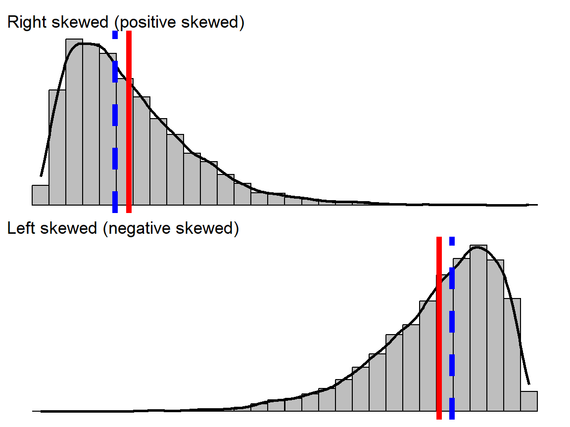
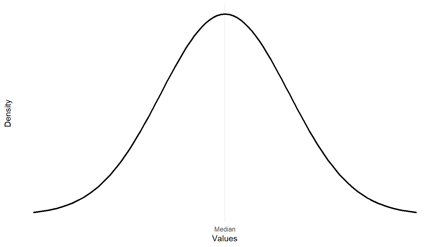
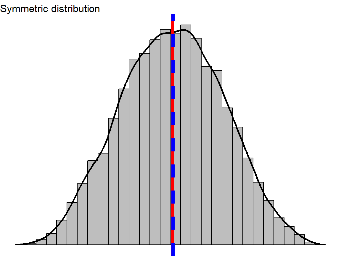
Symmetric vs Non symmetric

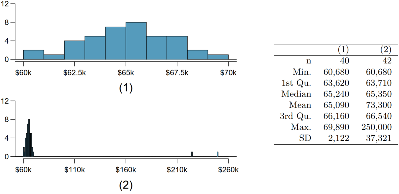
Extreem and influential observations

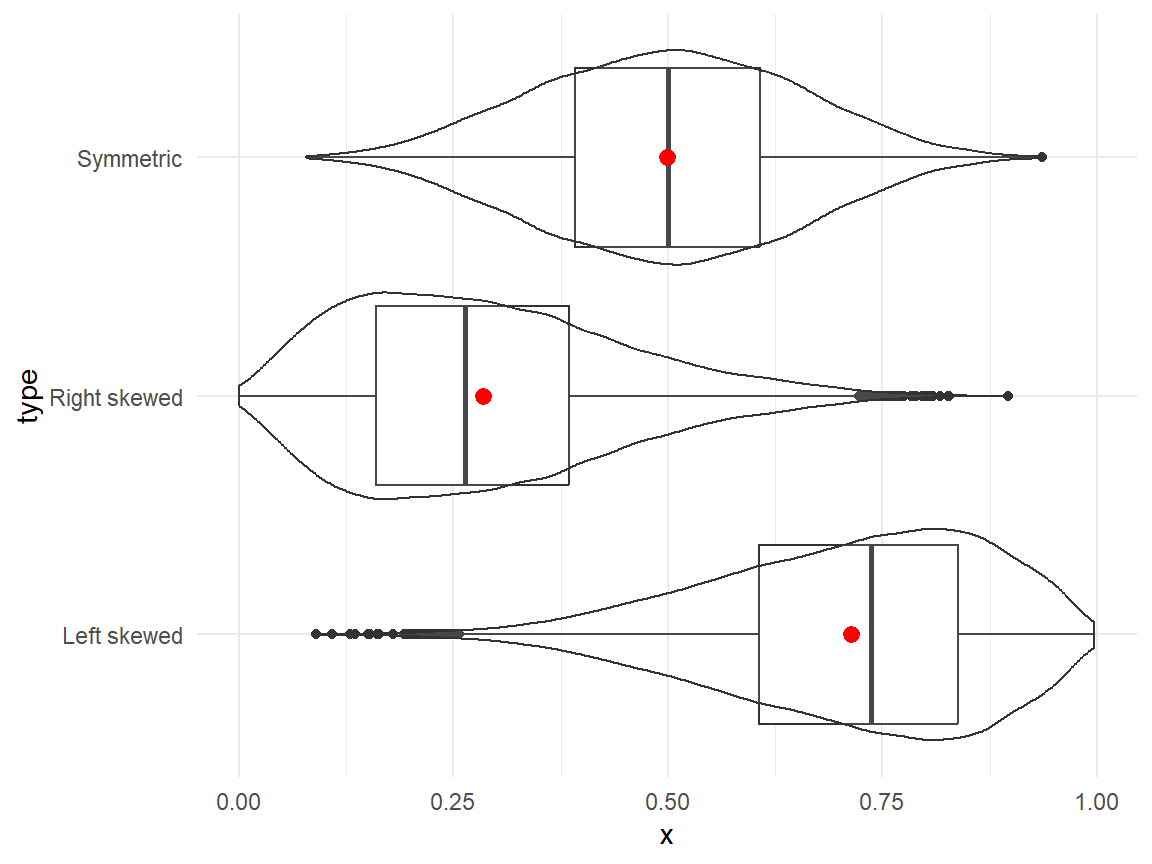
• Mean is heavily affected by influential observations.

• Median is more robust.

Cumulative Distribution

• Show all the data points at once with their contribution to the distribution of the value x

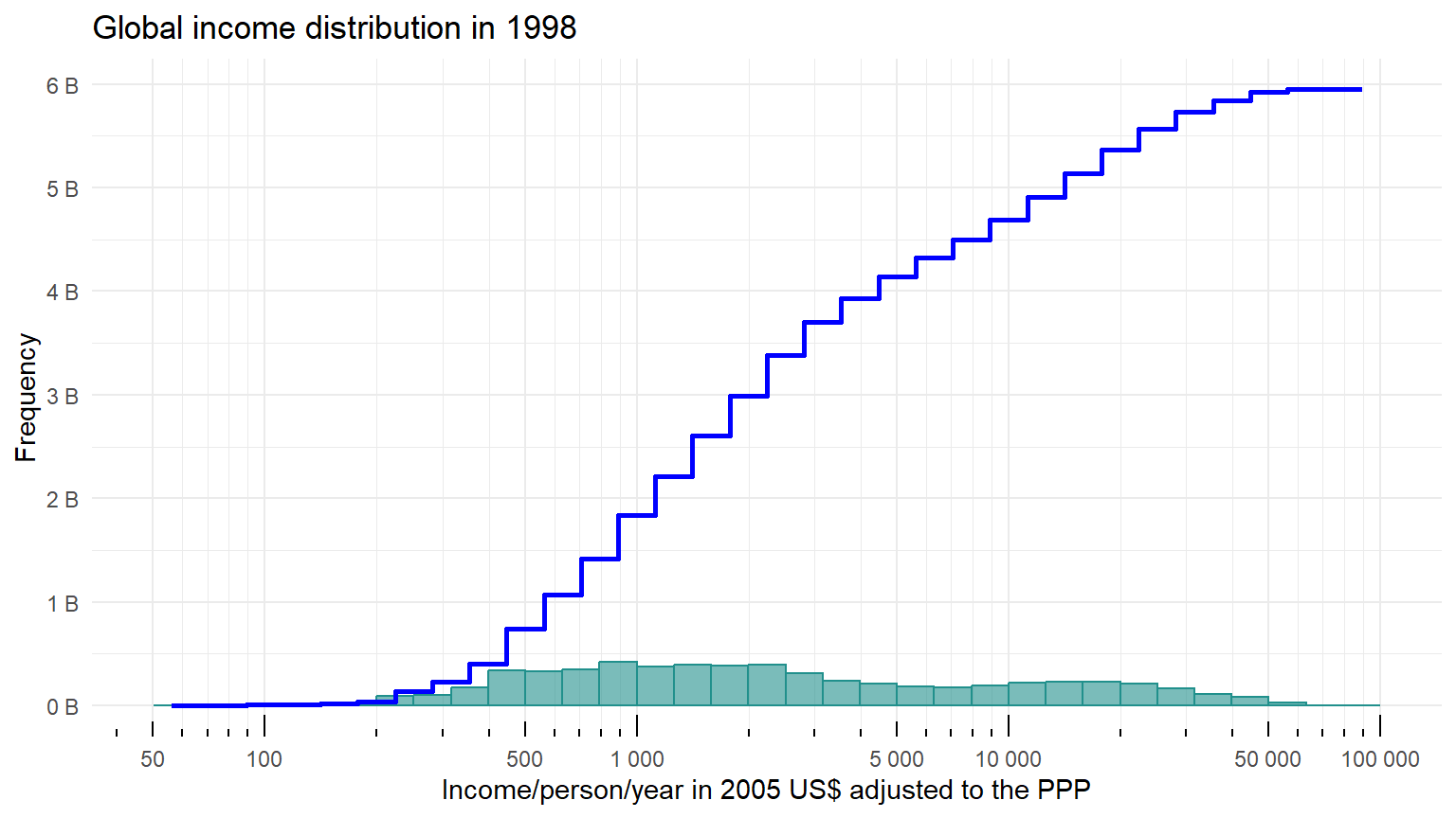
• See Ch. 8 Visualizing distributions: Empirical cumulative distribution functions and q-q plots in Fundamentals of Data Visualization (Wilke 2019)

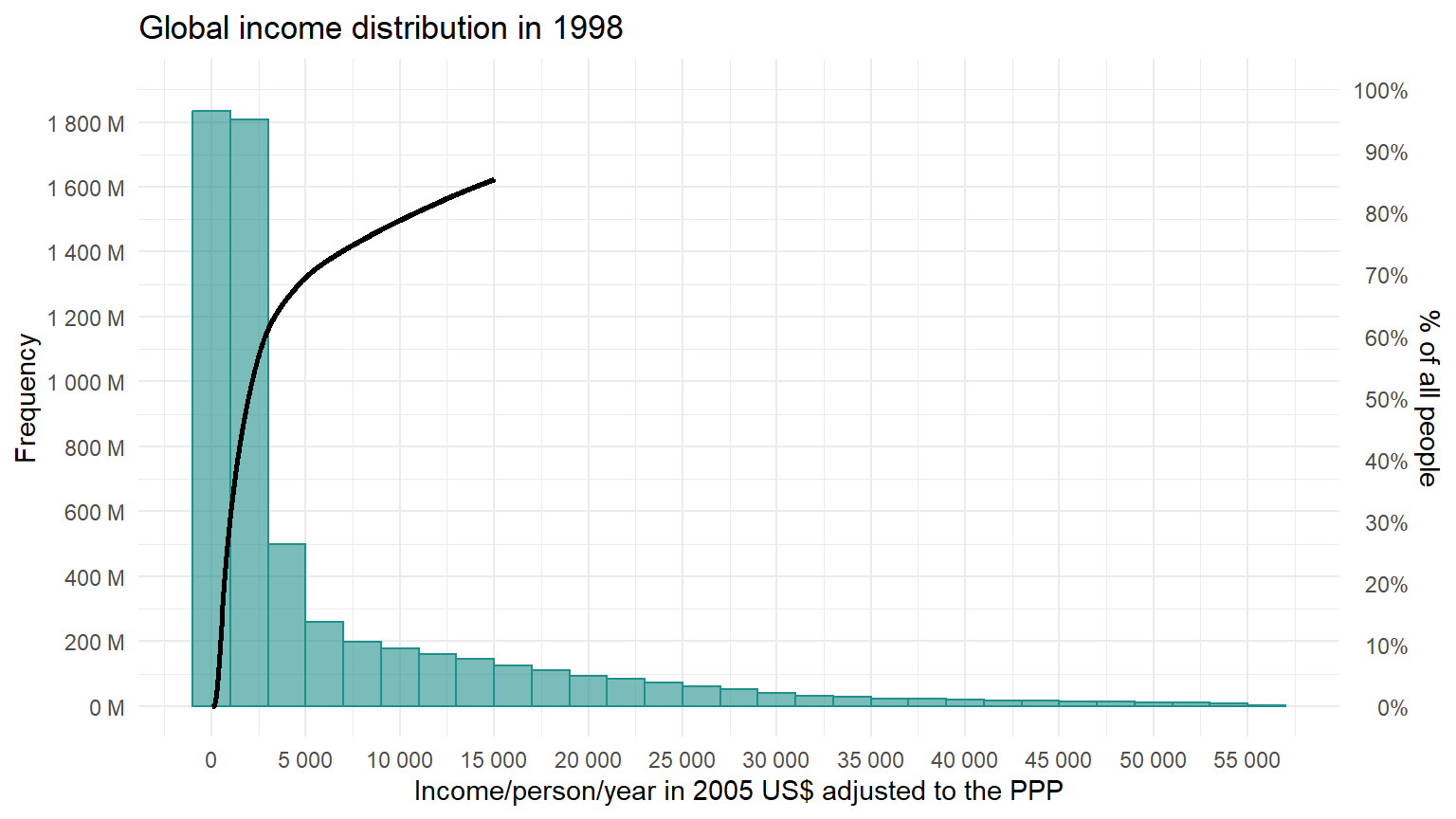
From a density to a cumulative distribution

How to:

• Order all observation ascendingly.

• Plot cumulative frequency for every existing observation on Y axis.

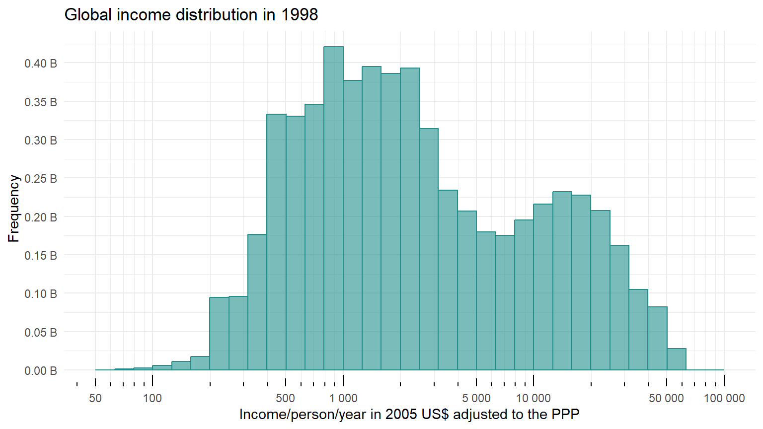
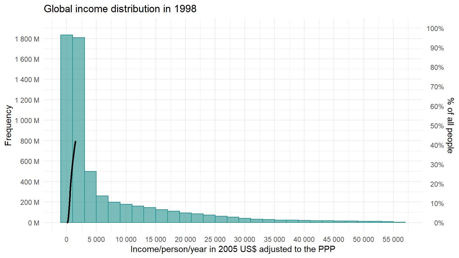
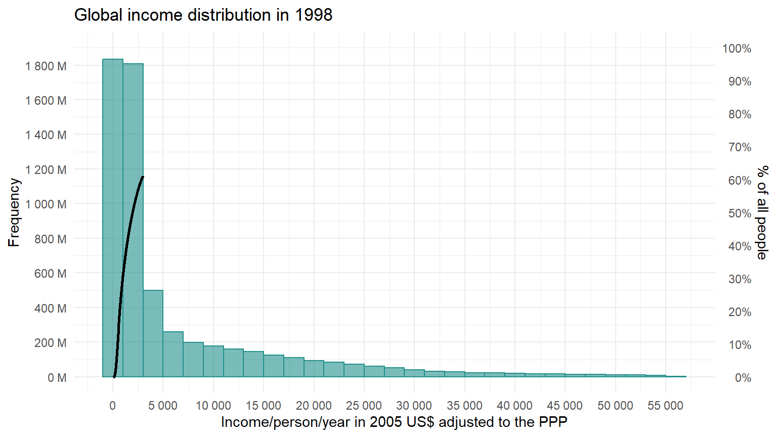
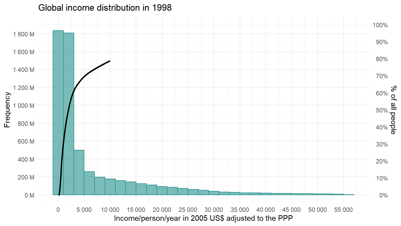
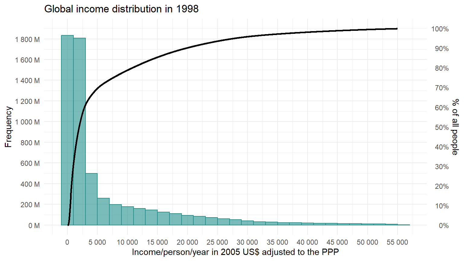
Cumulative distribution of income (1)

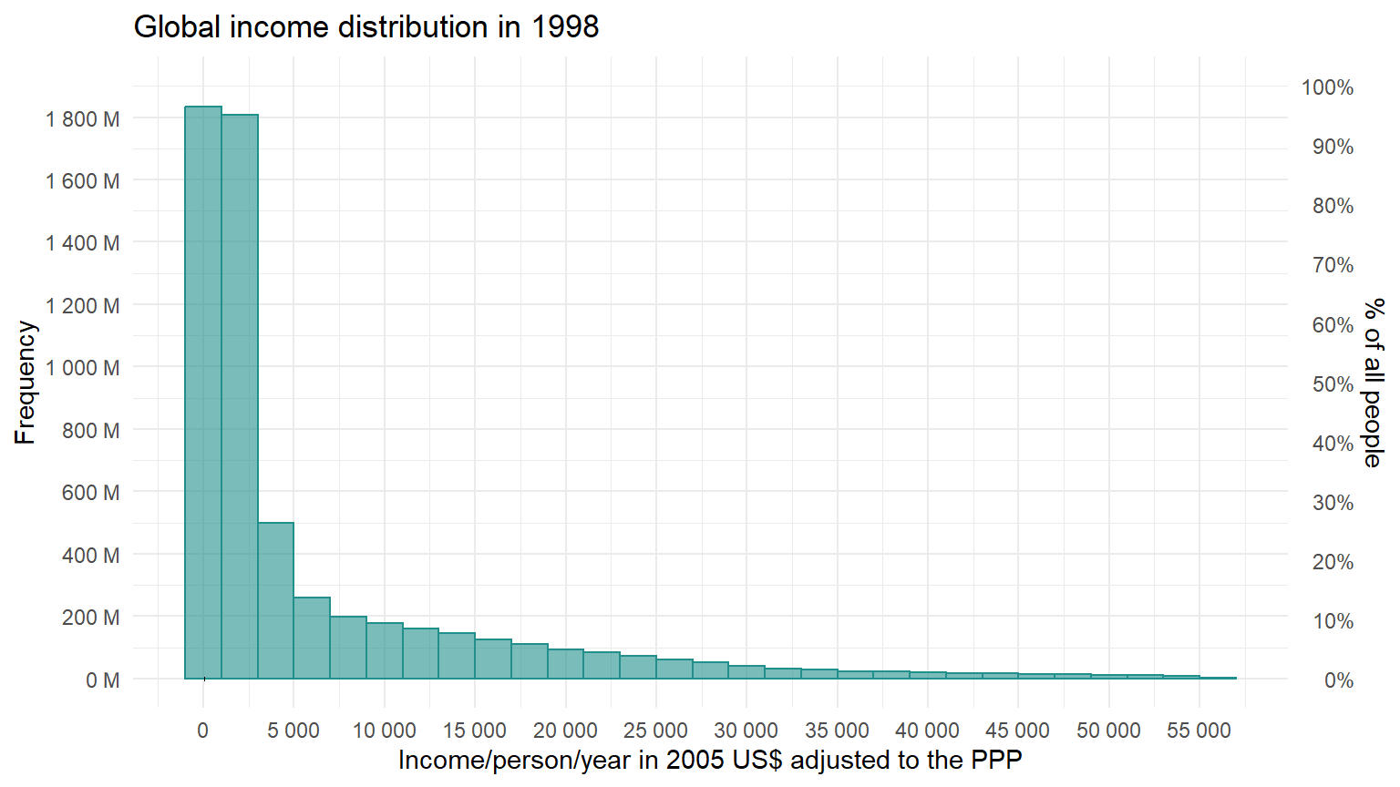
Cumulative Distribution: applications

Measuring income inequality

Income inequality

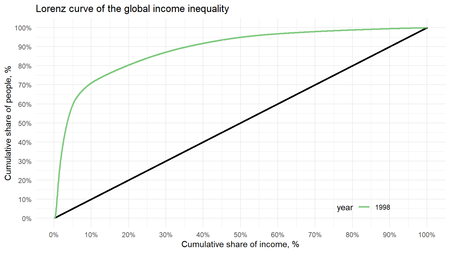
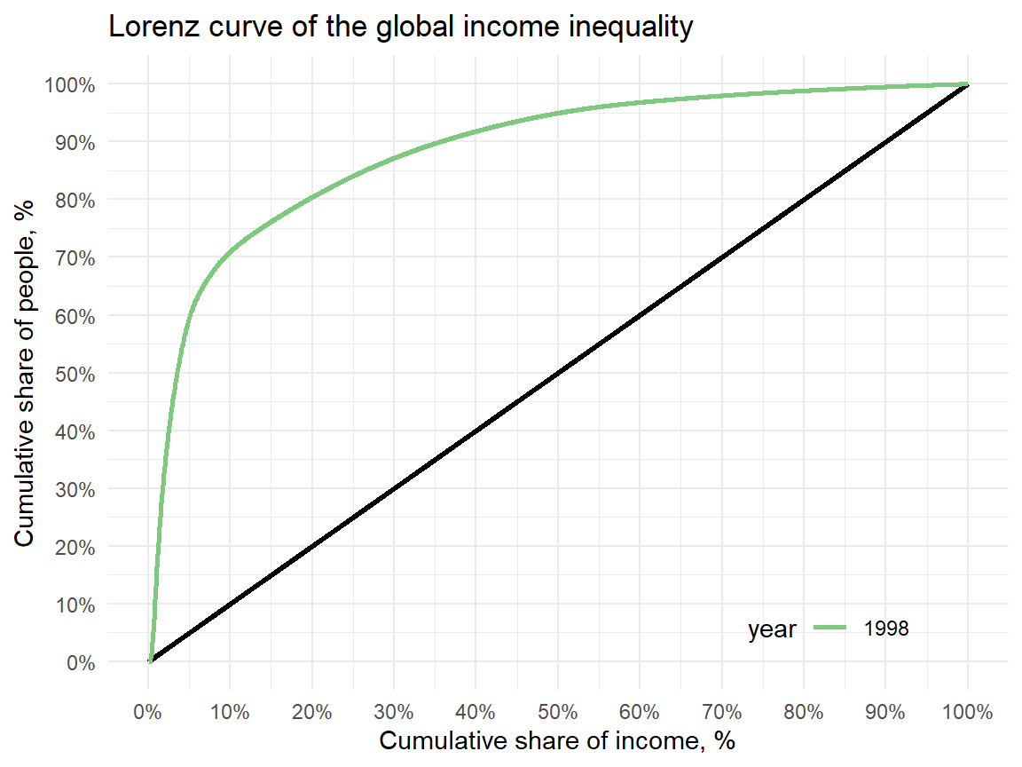
Lorenz curve

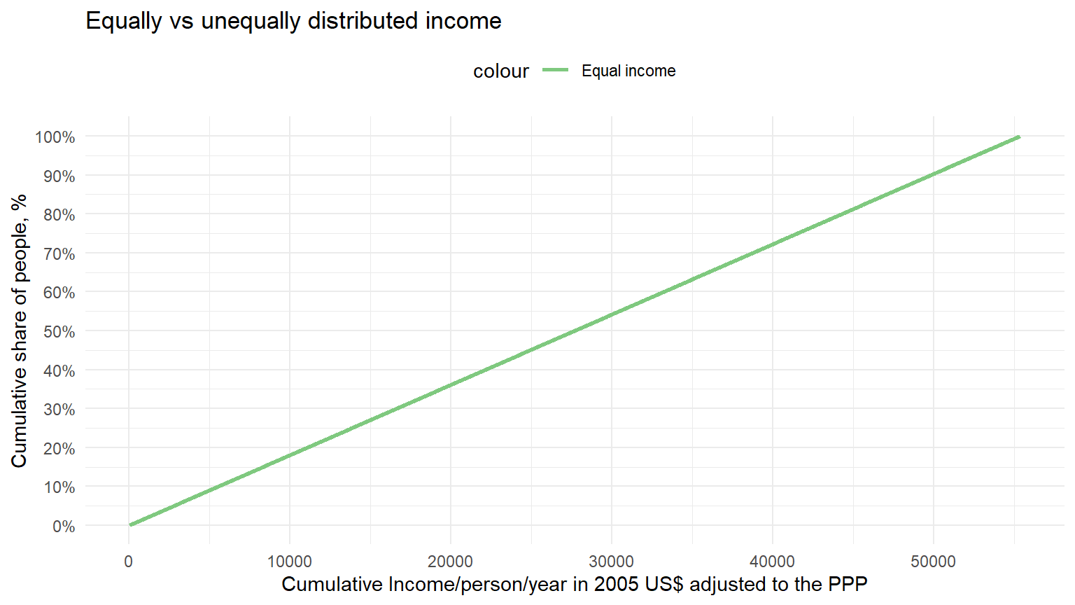
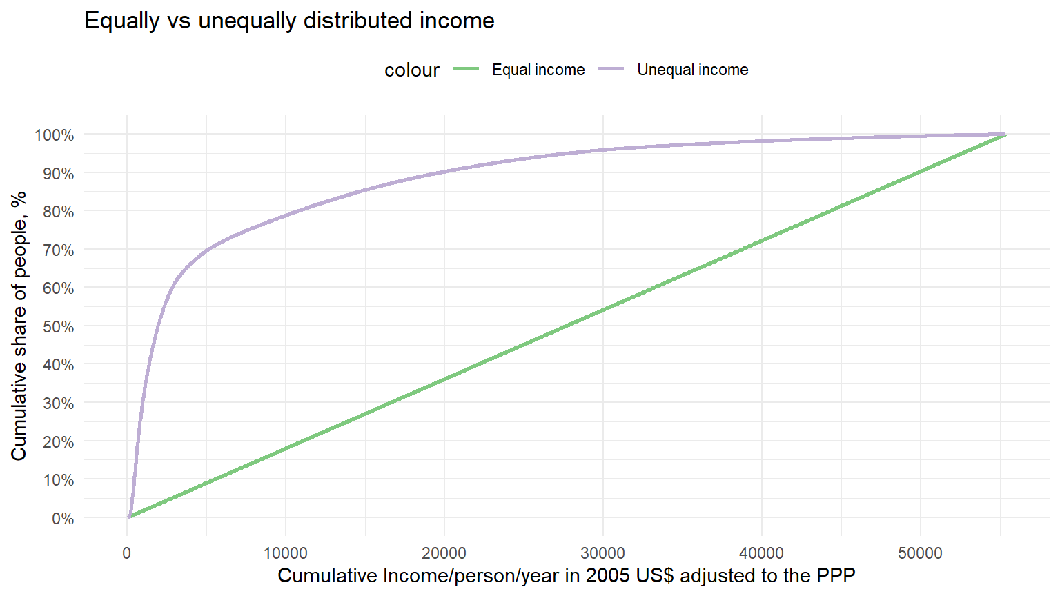
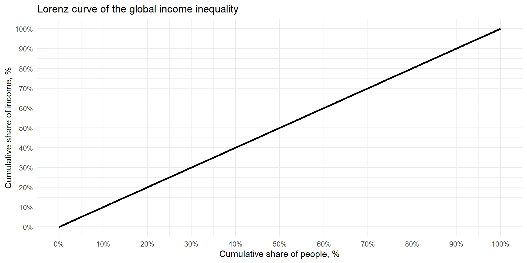
The Lorenz curve:

• Is a cumulative distribution

• Arrange all individuals by increasing income

  • from 0% to 100% of maximum income.

• Compute cumulative % of people by income level (0 to 100% of all people).

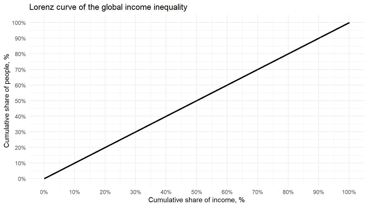
• see Graphical representation of the Lorenz curve.

How to read it?

Lorenz curve: spot any differences

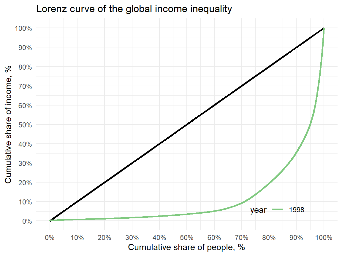
Example: Lorenz curve

• How has income distribution changed between 1988 and 2011?

• What statistical concept underlies the computation of the Lorenz curve?

• See also: https://ourworldindata.org/the-history-of-global-economic-inequality

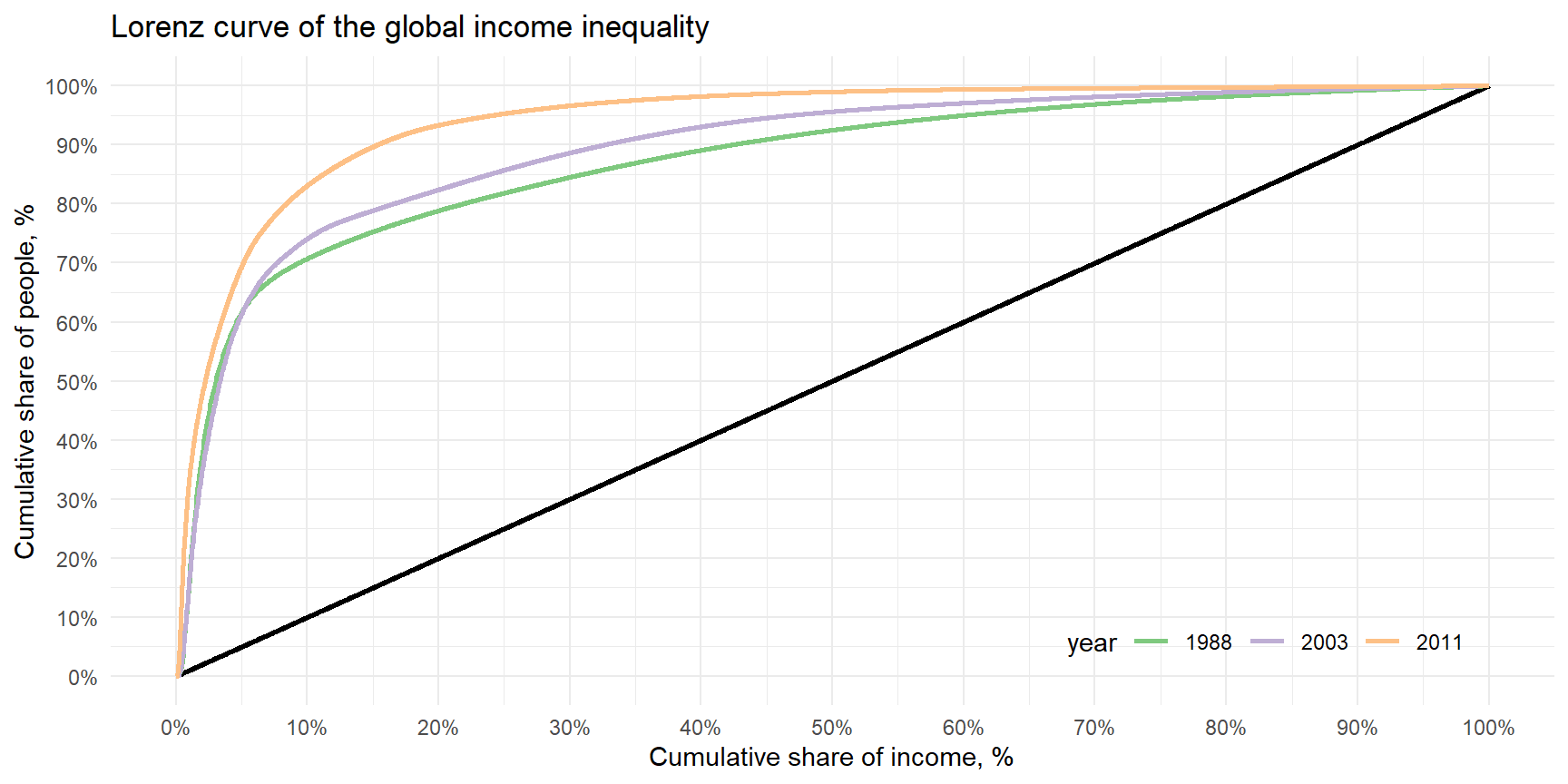
Homework examples

Lorenz curve

• Draw two Lorenz curves both with unequal income distribution.
• Explain differences between two curves?

At home: Read what is the Gini Coefficeint

Joe Hasell (2023) - “Measuring inequality: What is the Gini coefficient?” Published online at OurWorldInData.org. Retrieved from: https://ourworldindata.org/what-is-the-gini-coefficient [Online Resource]

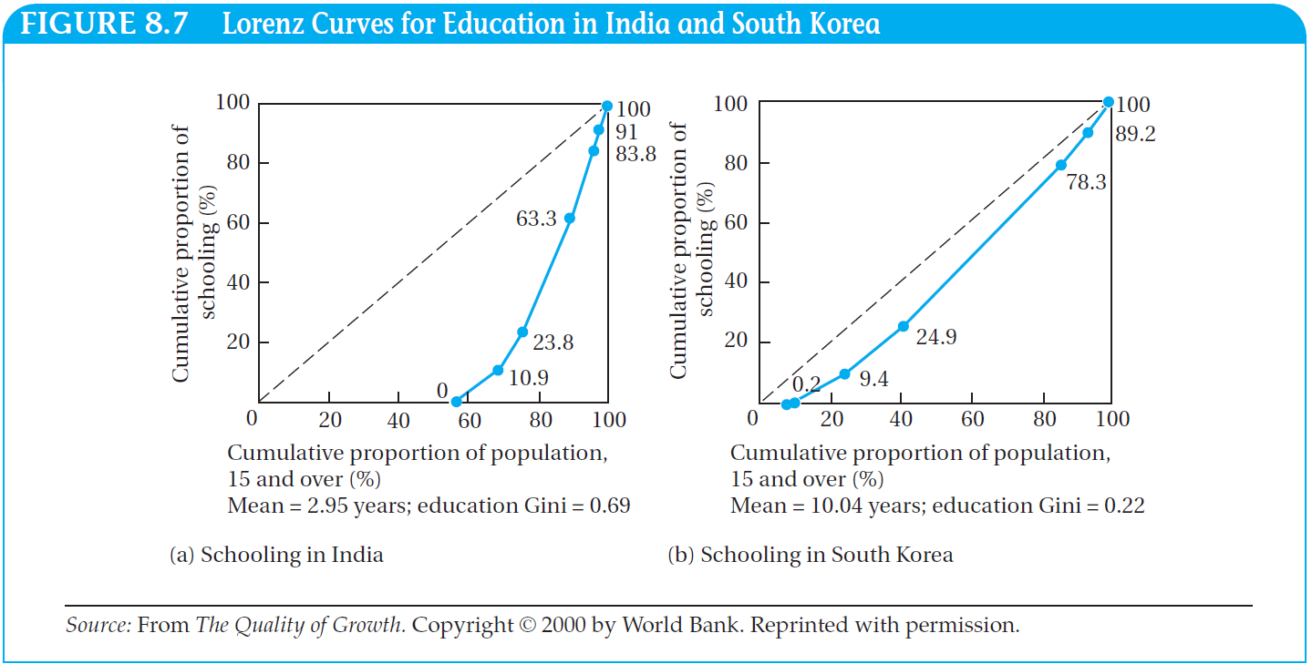
At home: Lorenz curve: Inequality

• What kind of plot is this?
• What does it show?
• Which of these two countries demonstrate more equal distribution?
• Why do you conclude this?

Variance

Variance

• Variance (\(Var[X]\)) is a measure of the spread of a distribution relative to its expected value (Dowdy et al. 2004)

  • is the measure of variability in a single variable;
  • is the average squared distance from the mean;
  • is in squared units (has no intuitive meaning);

• Standard Deviation (SD) is the squared root of the variance:

  • \(\text{SD} = \sqrt{\text{Variance}}\)
  • The standard deviation is
    • in the same units of measurement as the measured variable

Variance: population vs. sample

Population variance, \(\sigma^2\)

\[ \sigma^2 = \frac{\sum_{i=1}^N [x_i - \mu]^2 }{N}, \]

where \(\mu\) is the population mean:

\(\mu = {\sum_{i=1}^N x_i }/{N}\)

Only used with the population

Standard Deviation:

\(\sigma = \sqrt{\sigma^2}\)

Sample variance, \(s^2\)

\[ s^2 = \frac{\sum_{i=1}^N [x_i - \bar{x}]^2 }{N-1}, \]

where \(\bar{x}\) is the sample mean:

\(\bar{x} = {\sum_{i=1}^N x_i }/{N}\)

Most commonly used in statistics

Sample Standard Deviation:

\(s = \sqrt{s^2}\)

Standard Deviation

represents the “typical” deviation of observations from the mean.

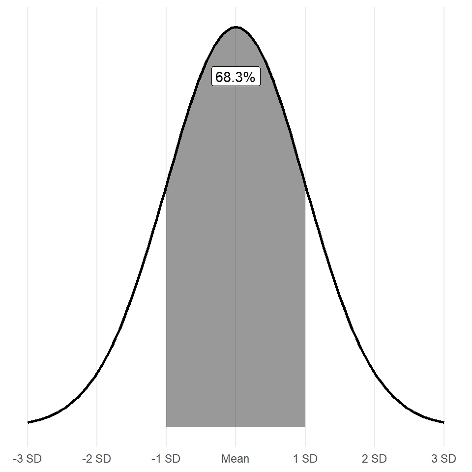
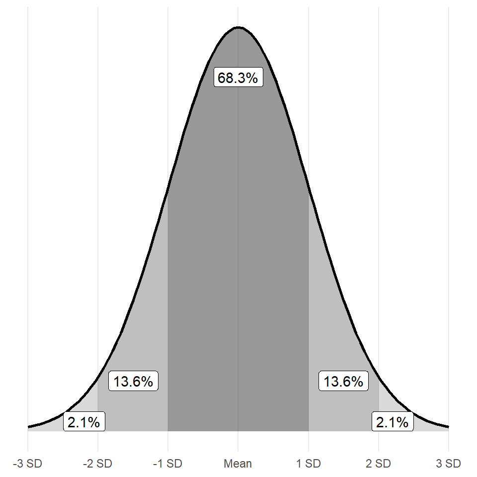
If the distribution is normal:

• 68.3% obs. are in +-1 SD;
• 95.4% obs. are in +-2 SD;
• 99.7% obs. are in +-3 SD;

The standard deviation is in the same units of measurement as the measured variable.

Not every distribution is normal, but SD can be the same

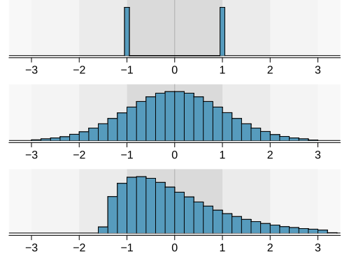
Note

A good description of distribution should include

• Central tendency;

• SD (Variance);

• Description of the shape;

  • modes

  • symmetry / skew

Quantiles

Quantiles

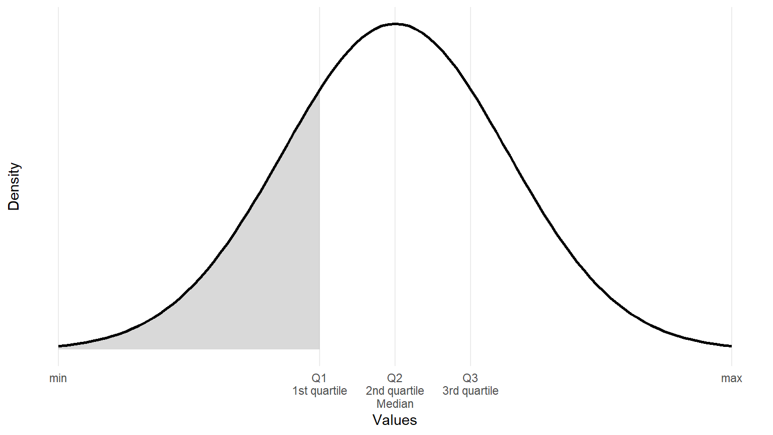
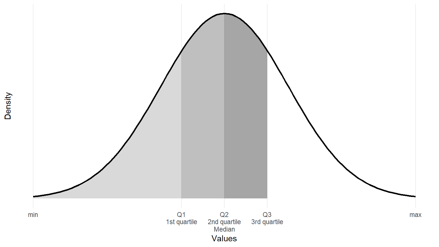
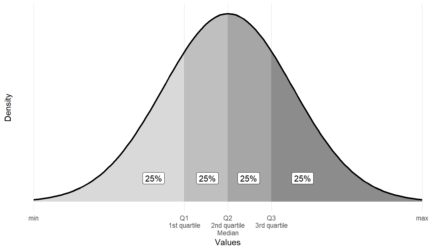
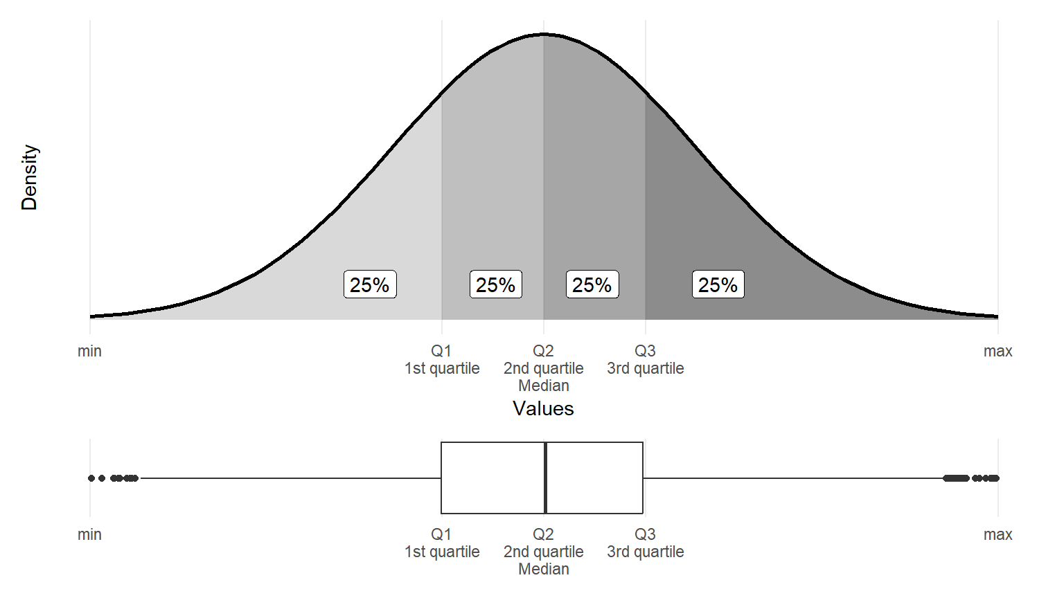
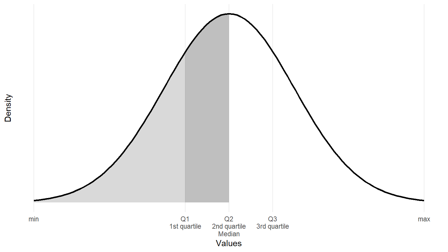
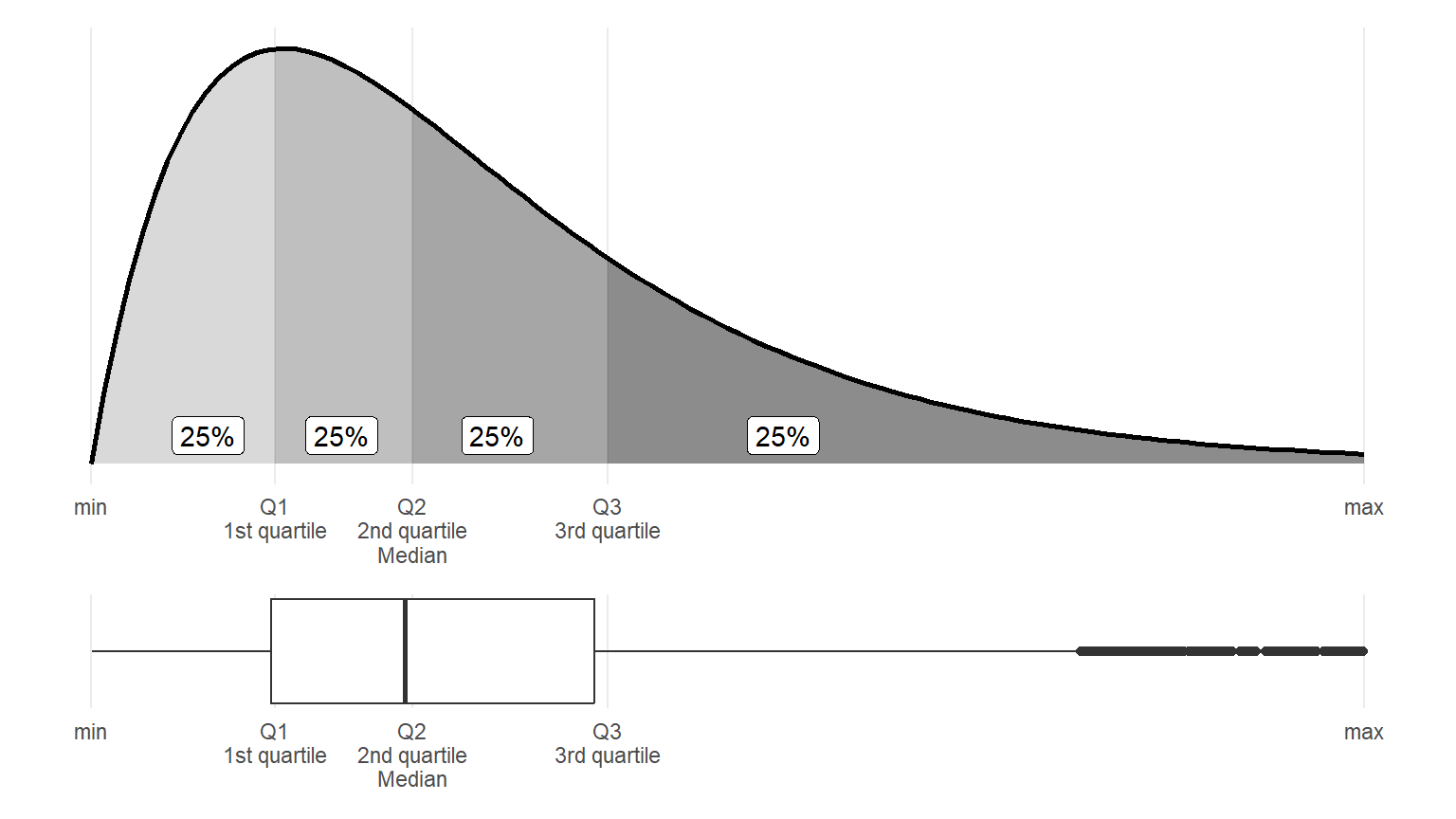
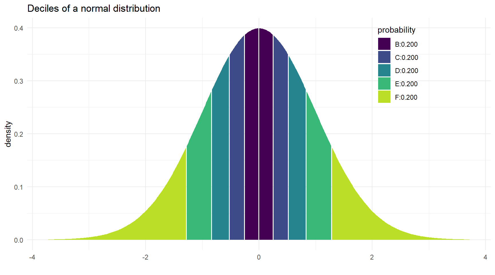
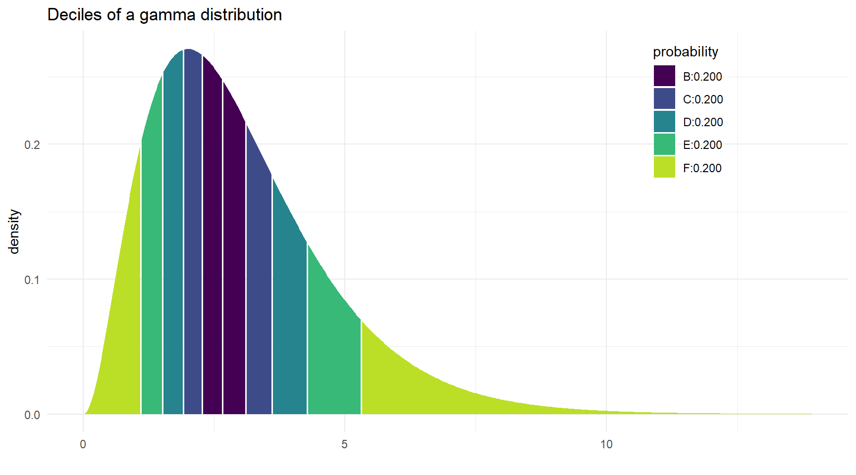
• cut points that divide our data into equal chunks with equal probability of being selected (equal number of observations in each chunk).

• Quantiles: Quartiles (4), Deciles (10), Percentiles (100)…

  • see Quantiles and Percentiles, Clearly Explained

• Range

• IQR - Interquartile range

Quartiles: every 25% of observations

Quartiles: non-normal distribution

Deciles: every 10% of observations (Normal)

Deciles: Gamma distribution

Example (1): income deciles

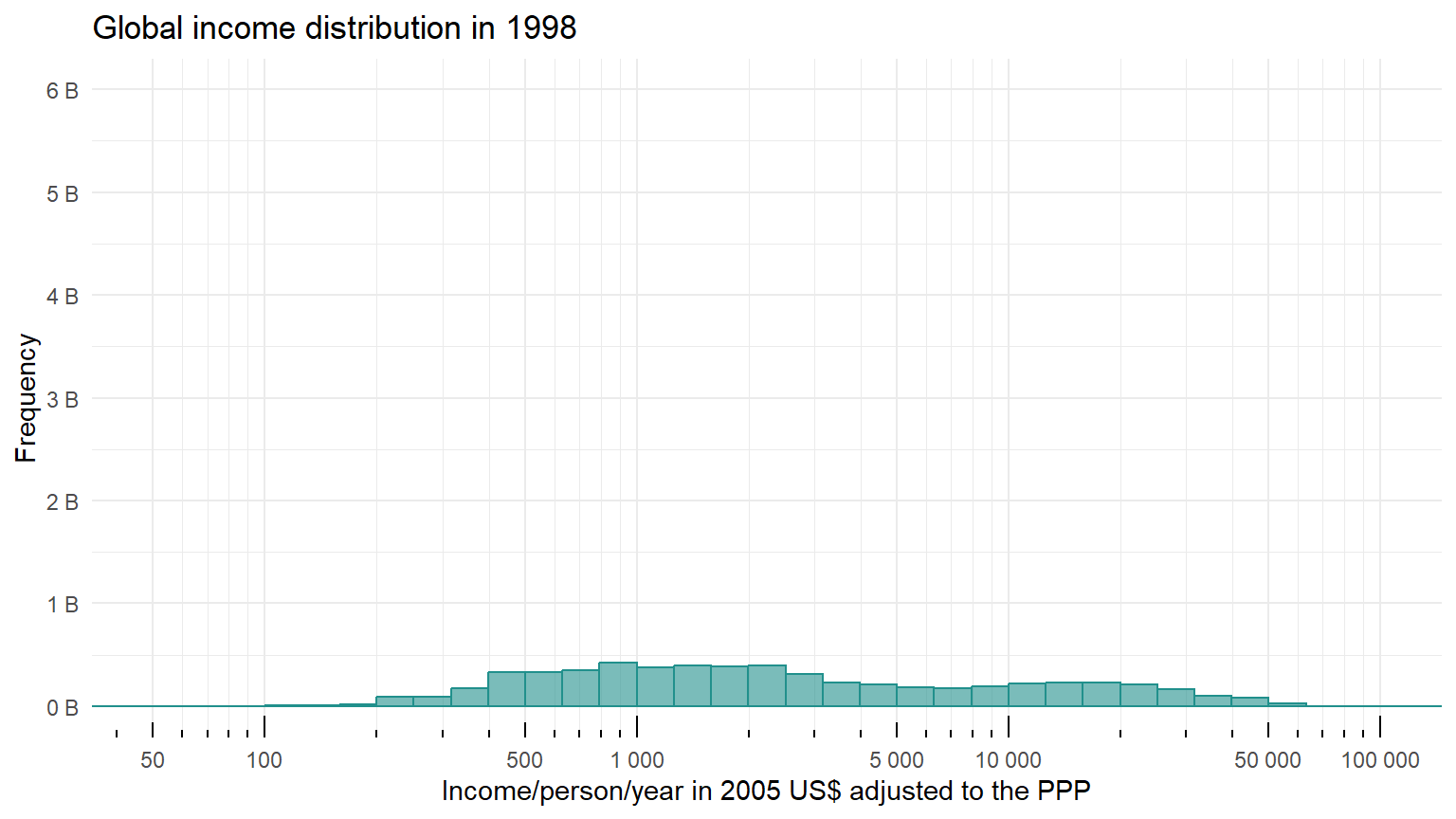
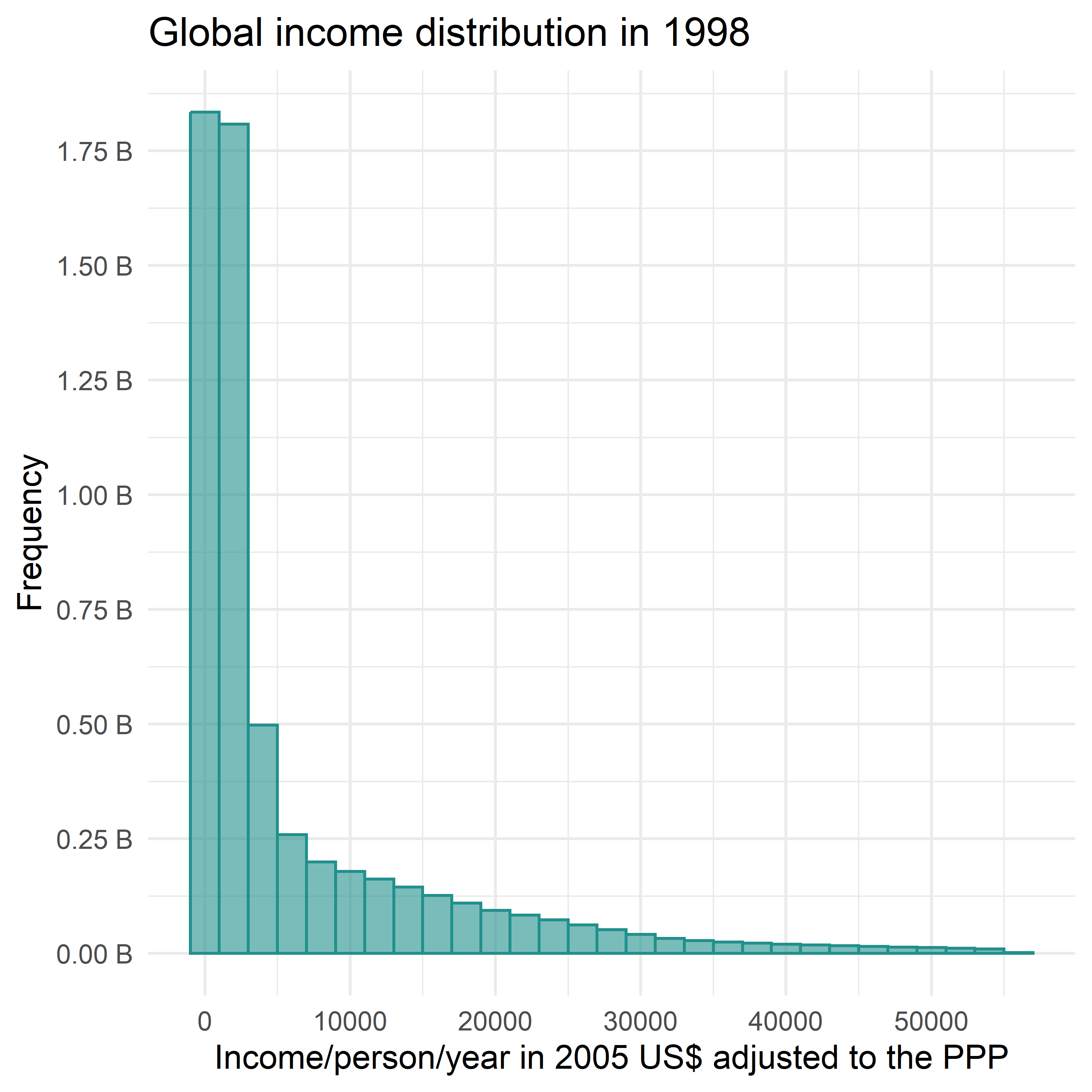
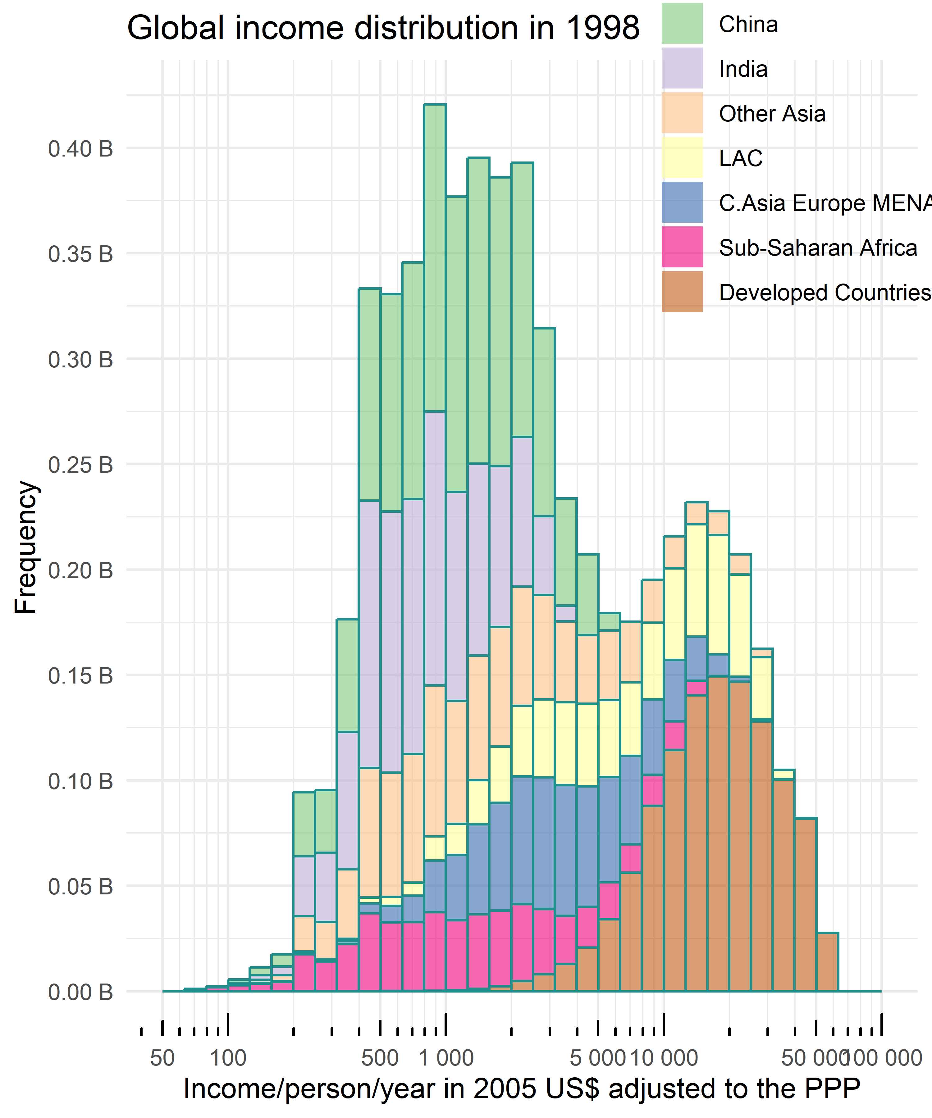
Deciles (1) of Income Distribution

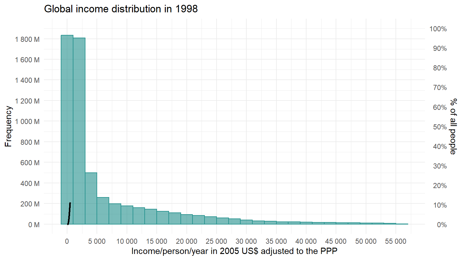
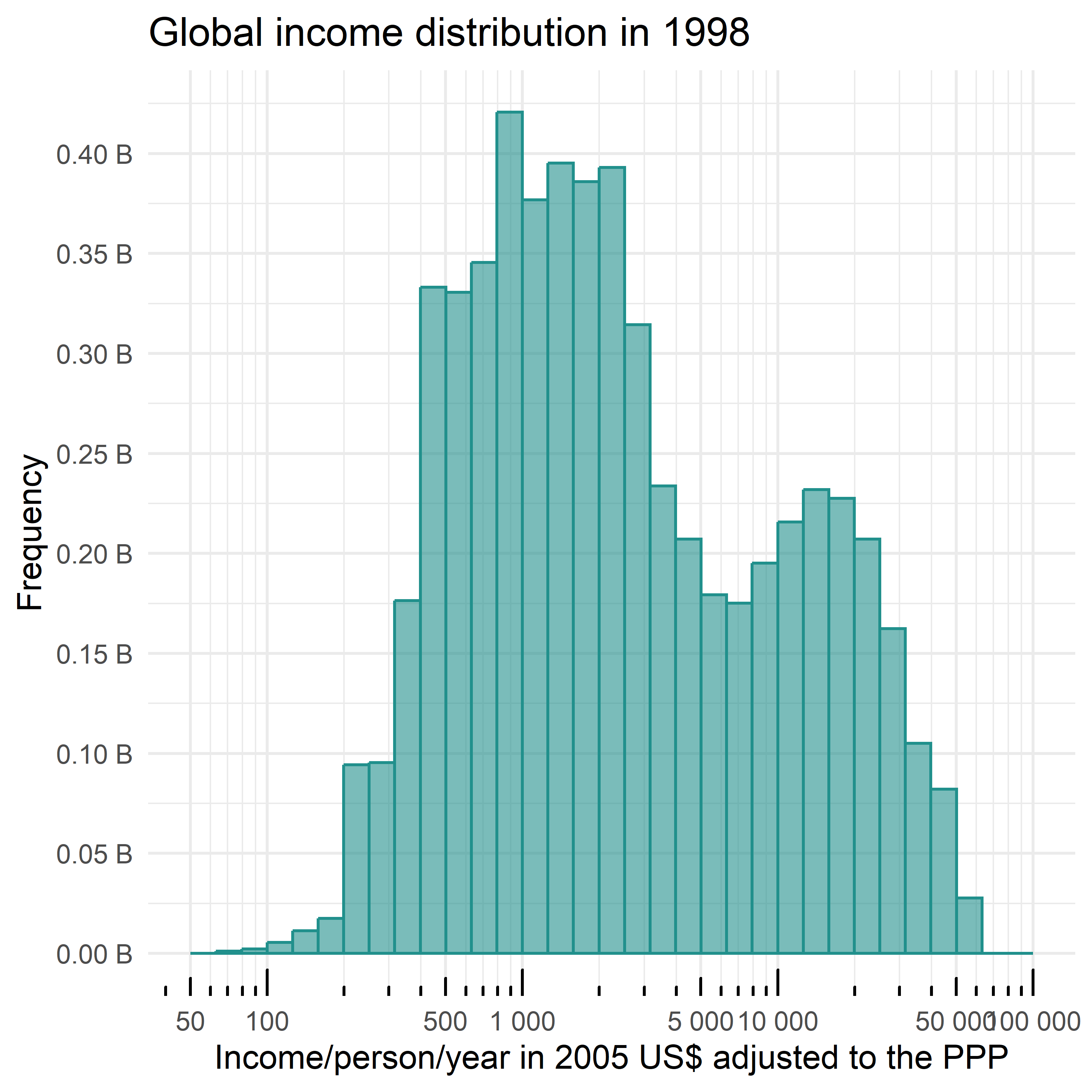
Deciles (2) of Income Distribution

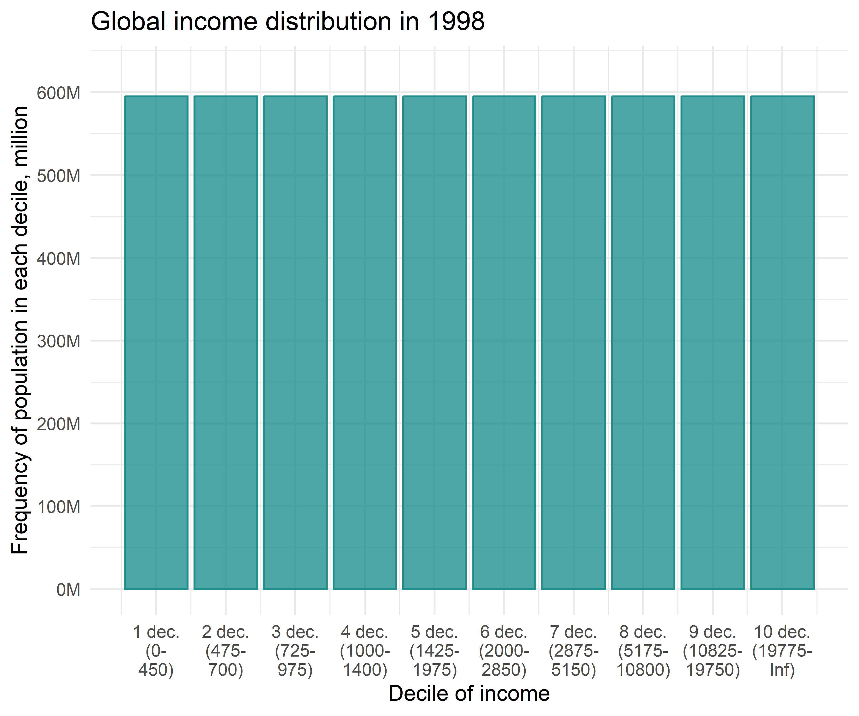
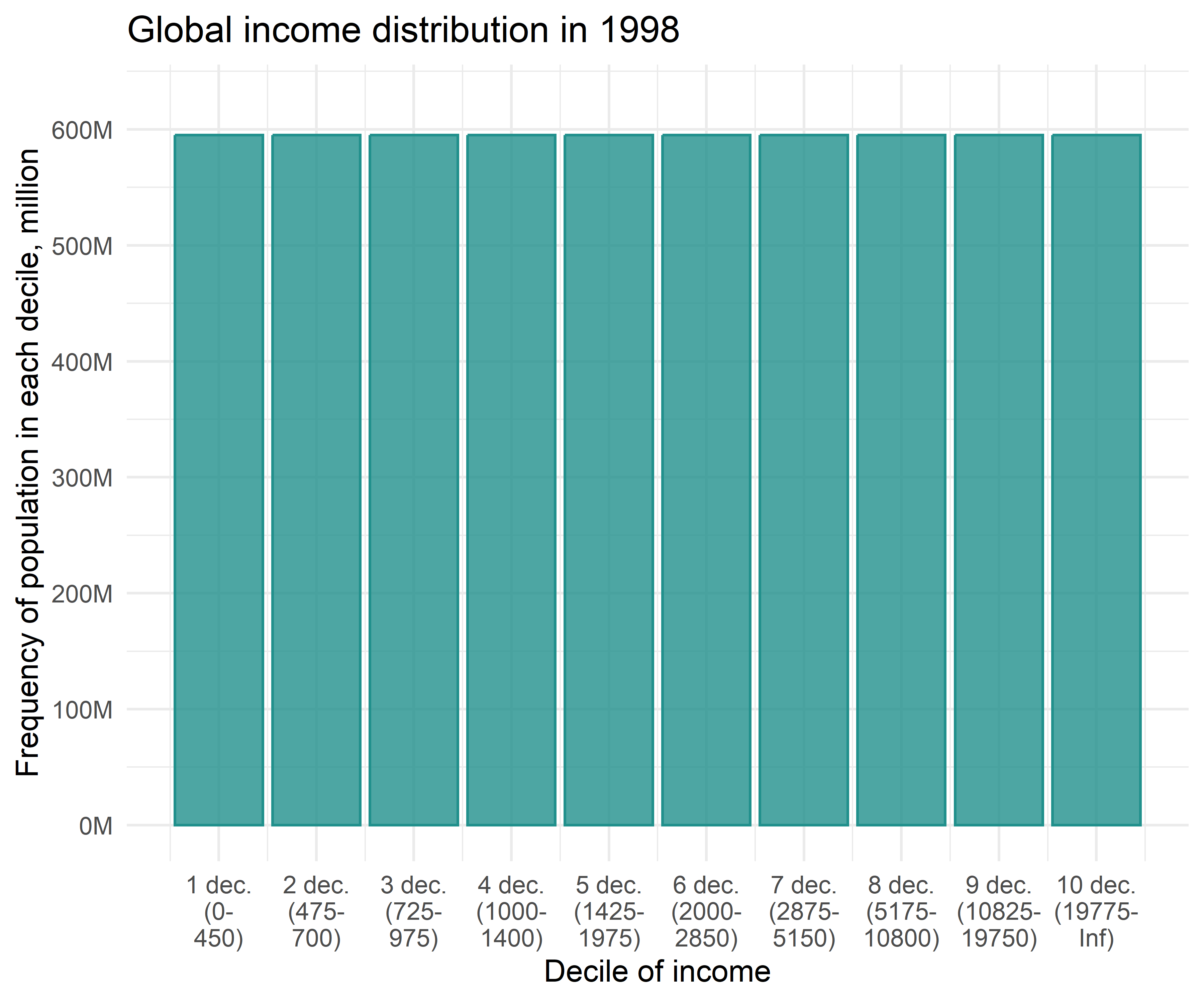
Let us draw a histogram with frequency by deciles!

• Note: the total population in 1998 was 6 billion

• Is it useful?

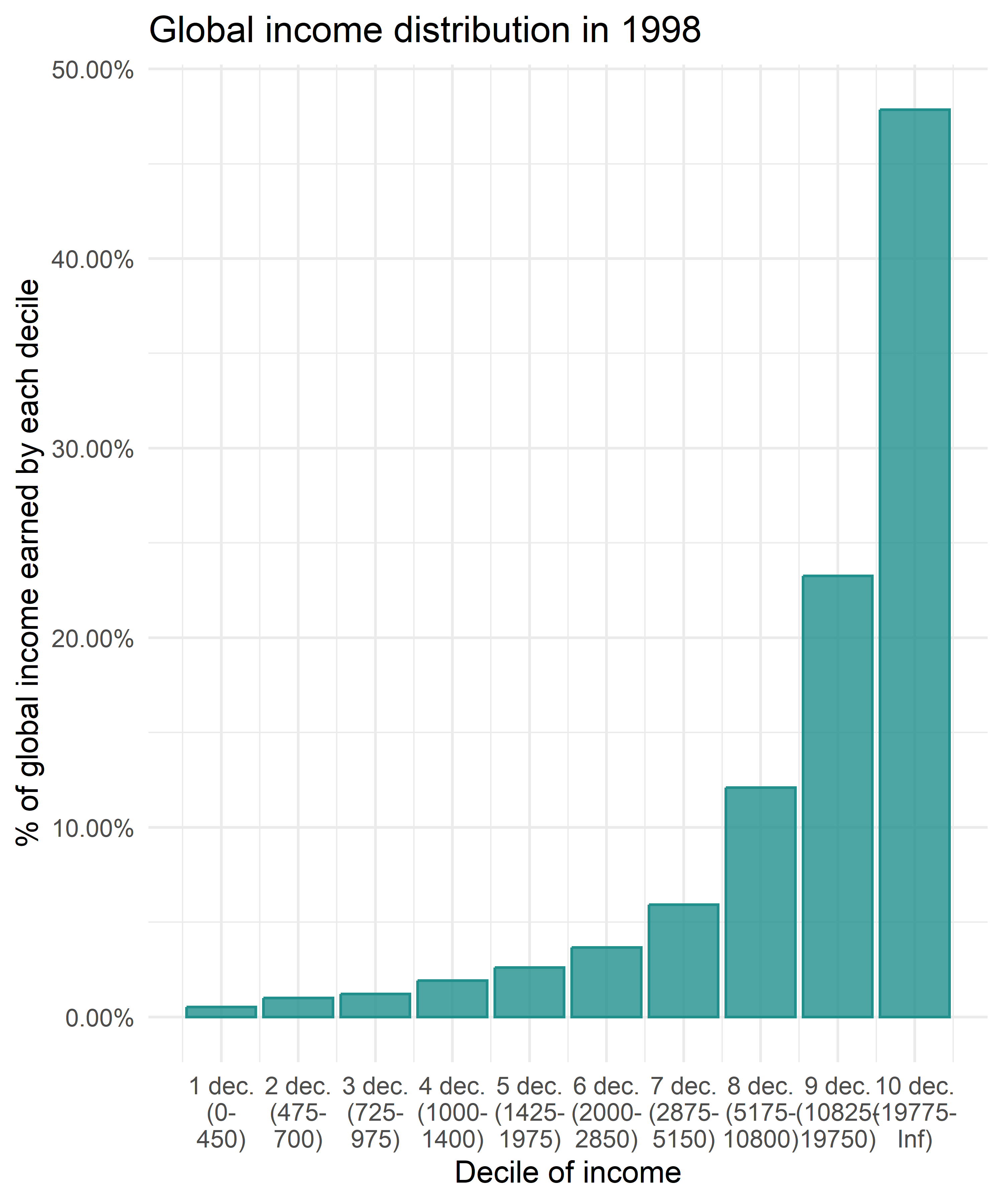
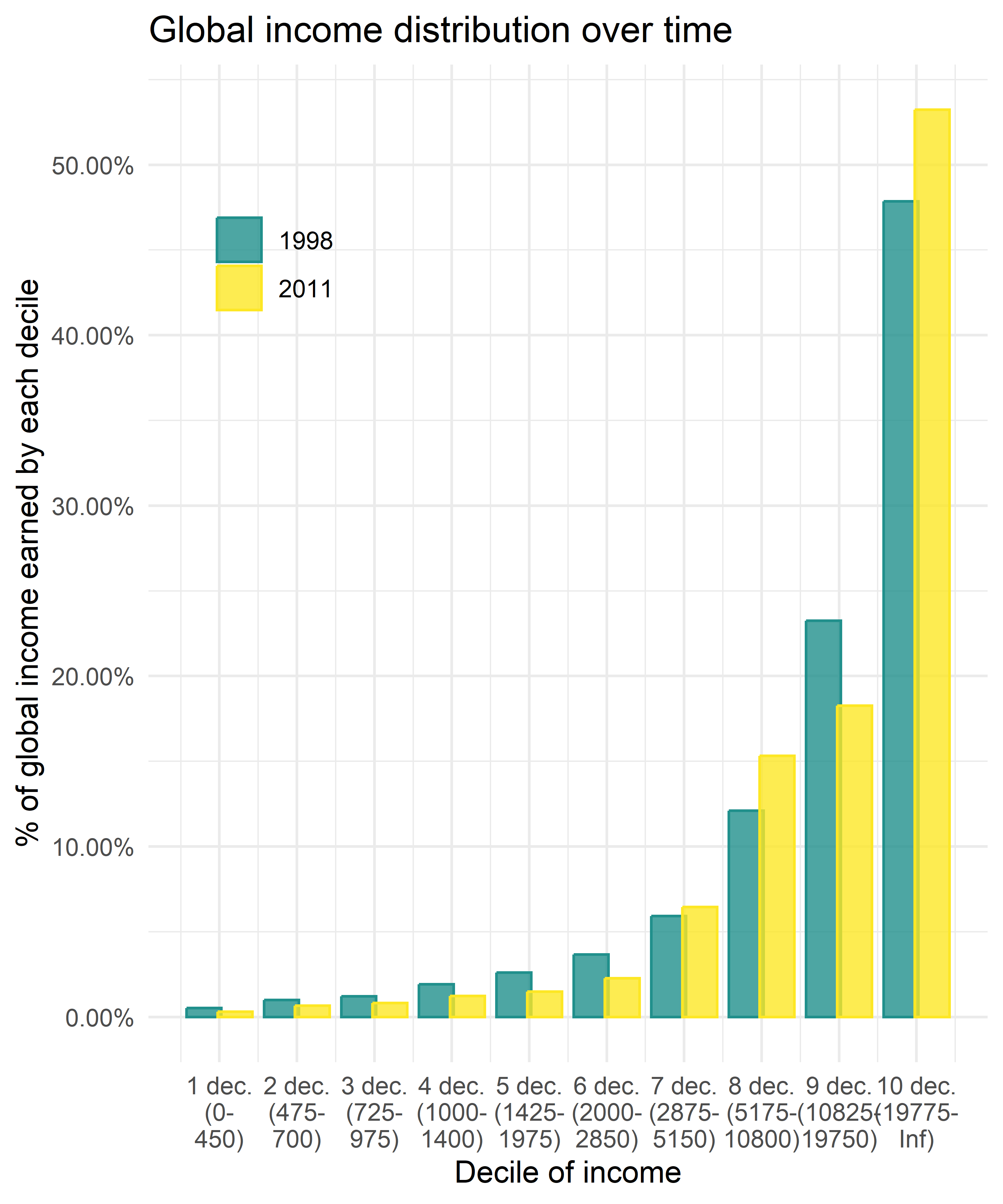
Deciles (3). New insights

Let us plot % share of total income on Y axis.

Deciles (4). New insights

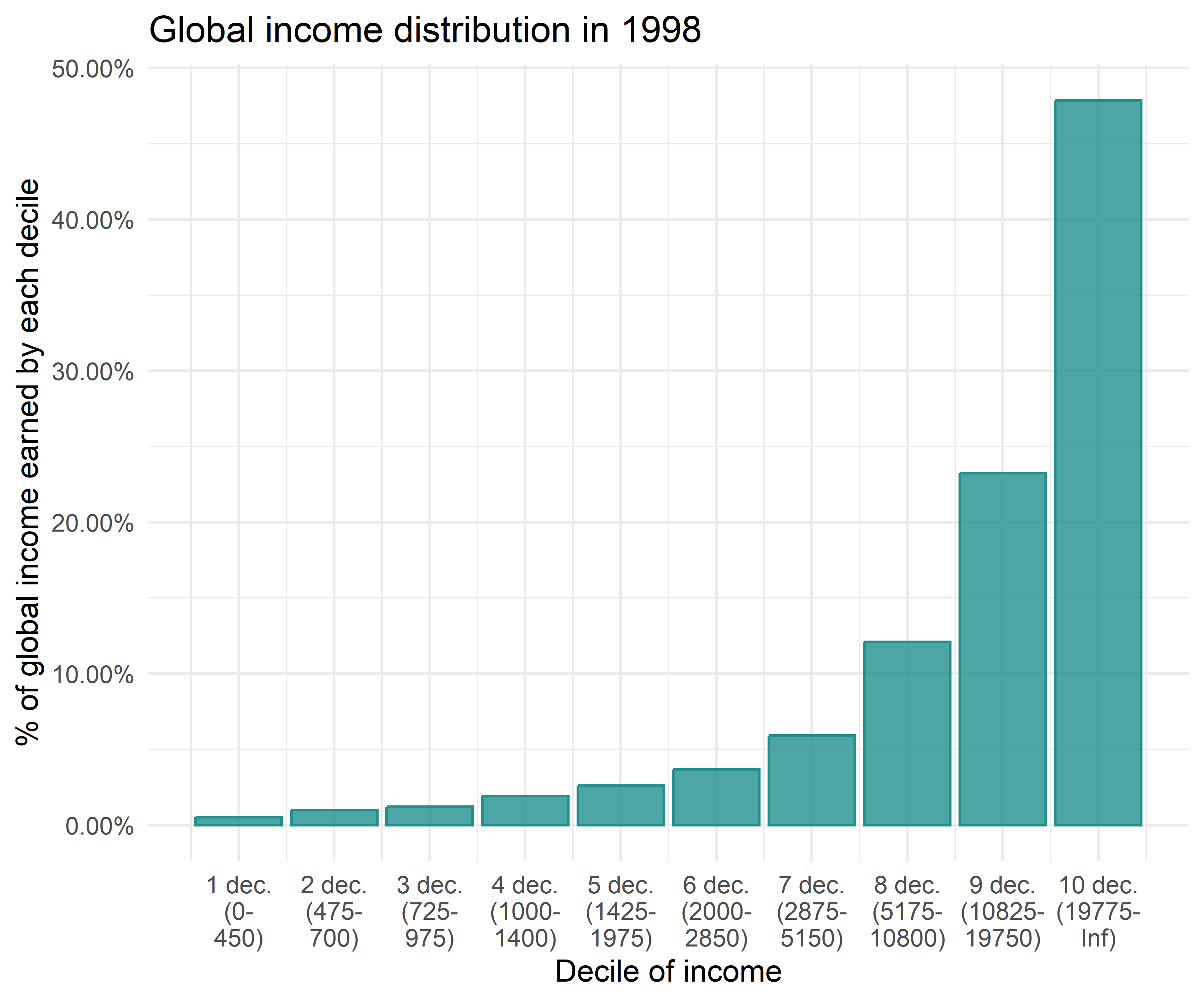
What does it show?

Where is the global income generated and distributed?

Deciles (5). Change over time

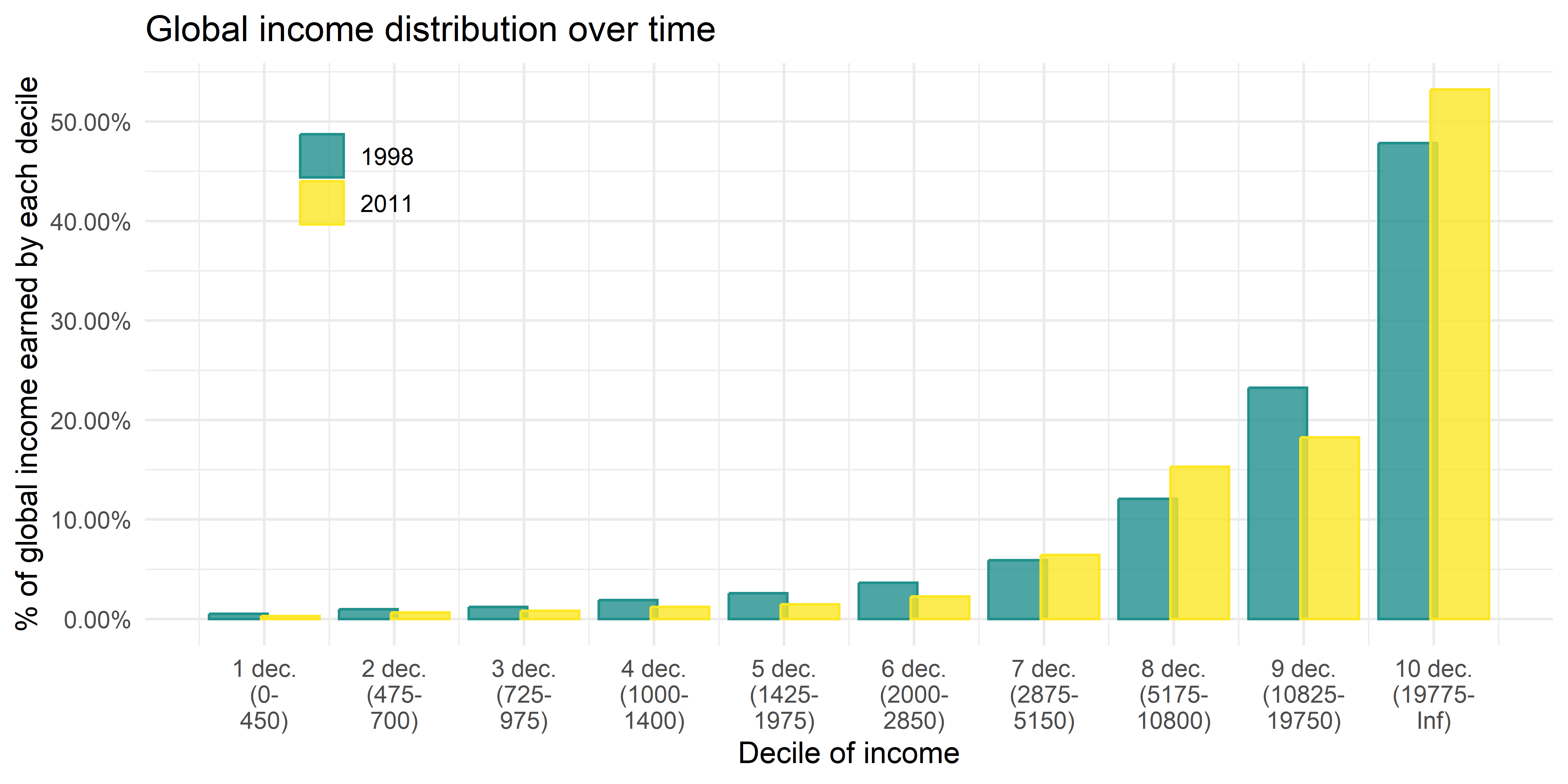
What had changed between 1998 and 2011?

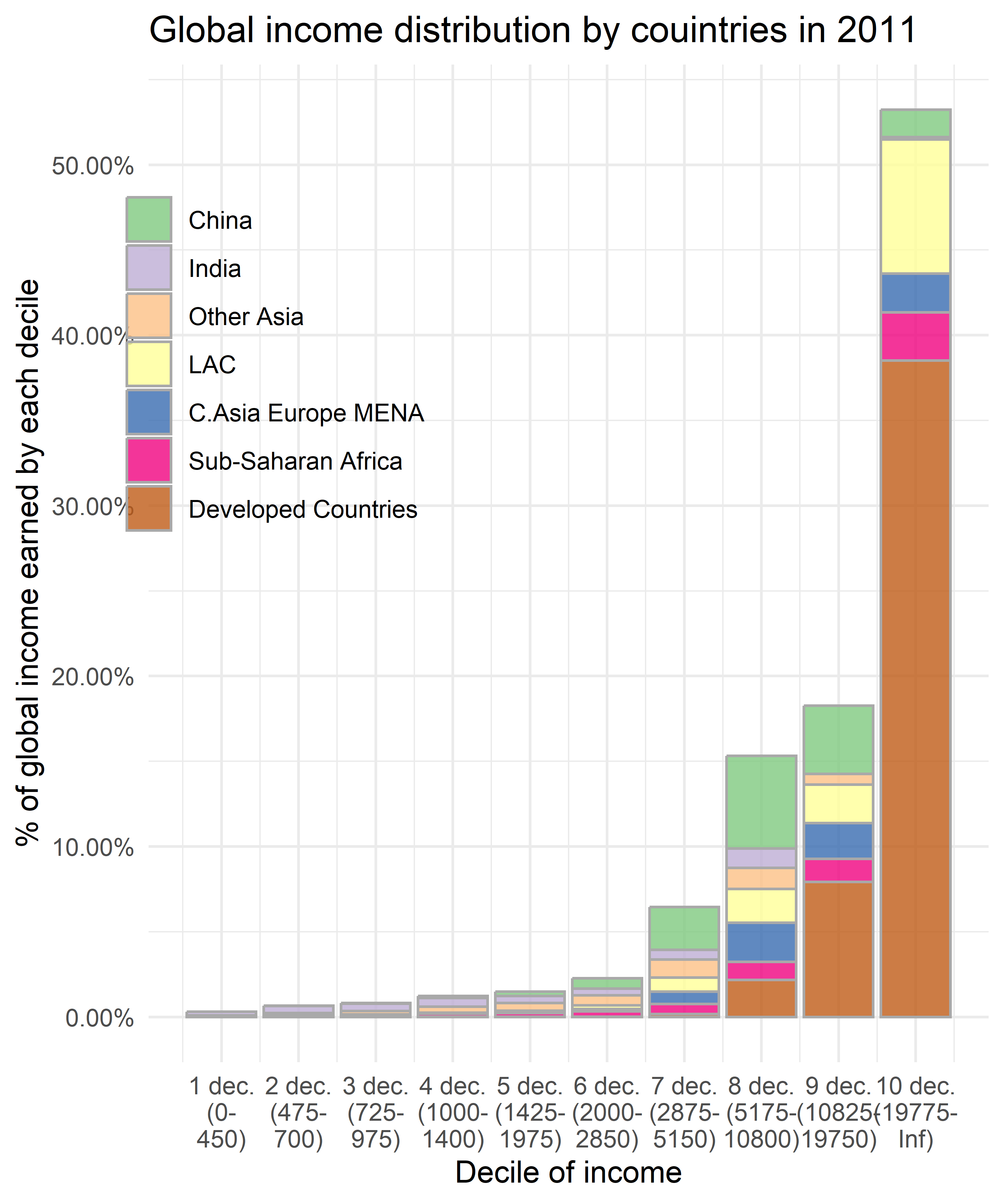
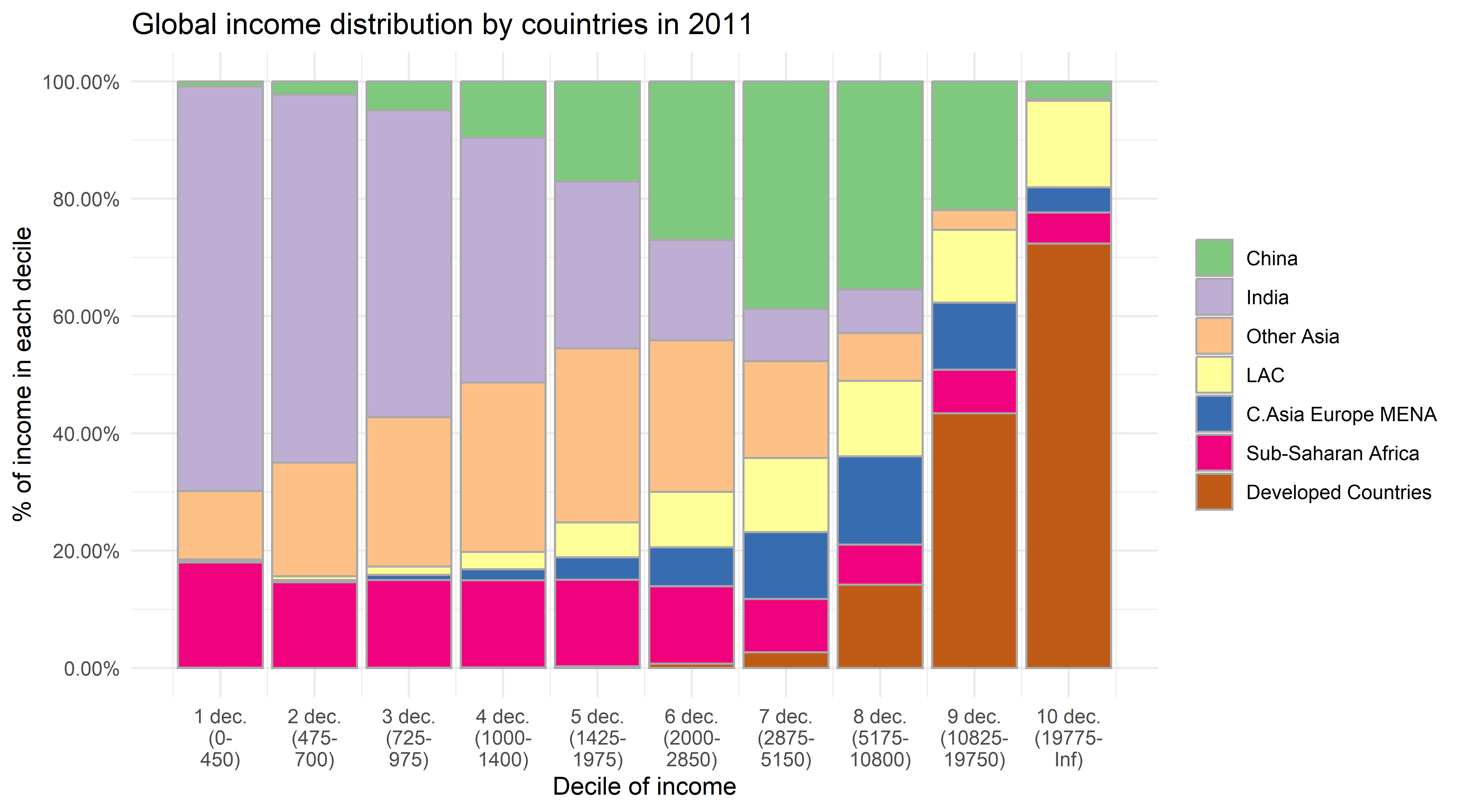
Deciles (6). By country

Deciles (7). By country

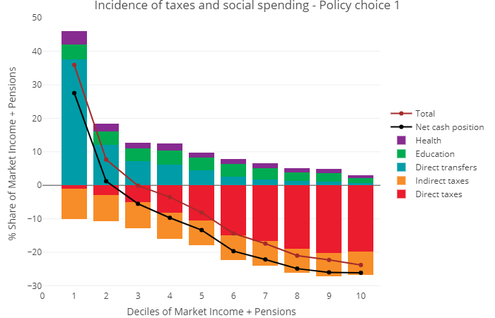
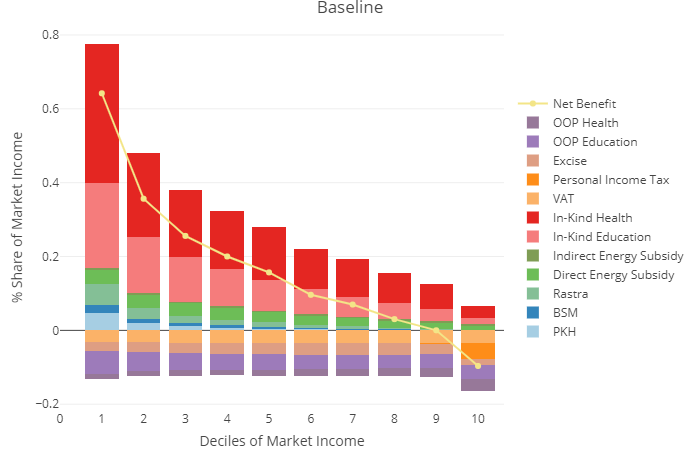
Example (2): inequality, taxes and subsidies (1)

Fiscal policy can redistribute income

• Taxes could be ‘collected’ from the ‘rich’:

  • Direct taxed: income tax
  • Indirect taxed: VAT, and excises

• Subsidies could ‘distribute’ wealth to the ‘poor’:

  • Direct subsidies: unemployment benefits, child support
  • In-kind subsidies: health and education

• See: https://commitmentoequity.org/

The Data

Data below is produced based on the representative HH surveys.

• For each individual income by sources and expenditure by cause are calculated.

• Then individuals are aggregated into the deciles of income.

• Each individual earns market income, while taxes and subsidies subtract or add to it.

Progressive taxation

Regressive taxation

Home work

Robust vs non robust variance

• Would the mean or the median best represent the central tendency?

• What does this say about the robustness of the two measures?

• Would the standard deviation or the IQR best represent the amount of variability in the incomes?

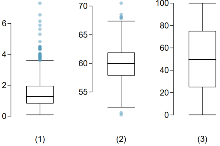
At home: Match distribution with the box plot

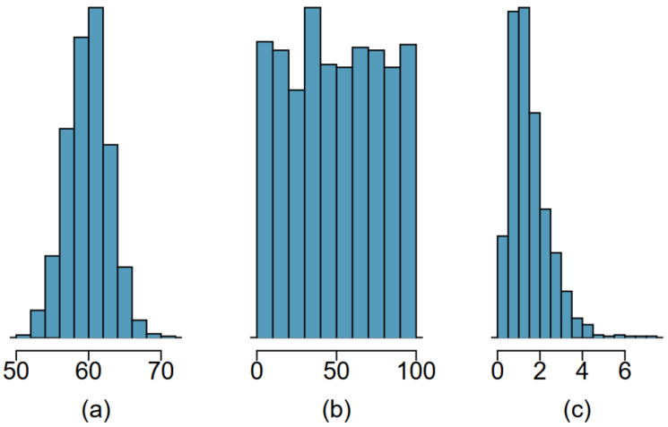
• Describe the distribution in the histograms below and match them to the box plots.

Application of variance in the descriptive analysis

Example: Measuring stunting

Important

Stunting is the impaired growth and development that children experience from poor nutrition, repeated infection, and inadequate psycho-social stimulation

• Stunting in the first 1000 days of life has negative consequences on the child’s physical and mental development.

• See: WHO. Stunting in a nutshell and more information on Hunger and Undernourishment.

Global Stunting

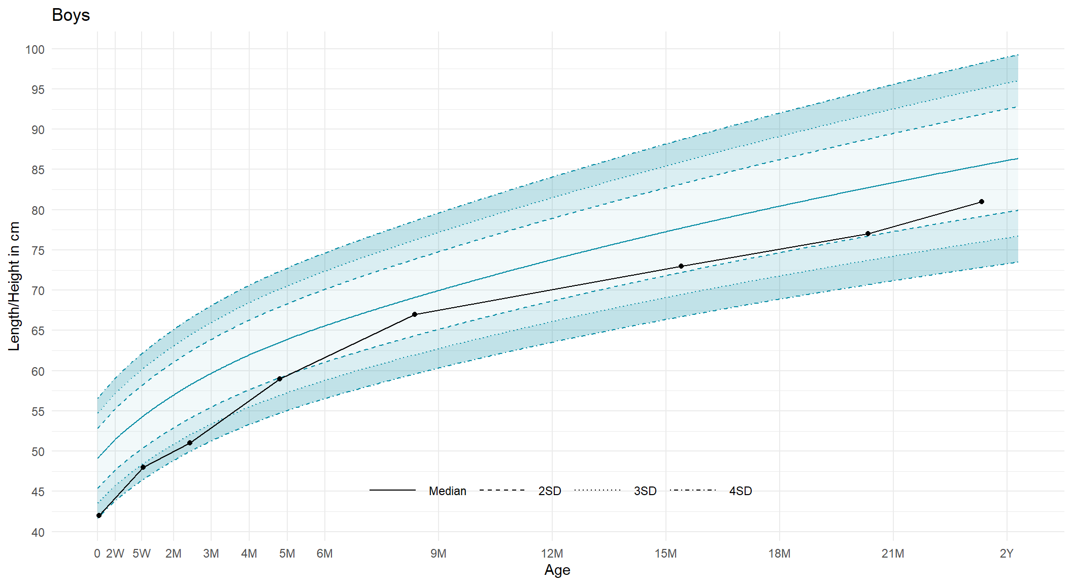
How to measure if the child is stunted?

WHO has developed:

• Child Growth standards

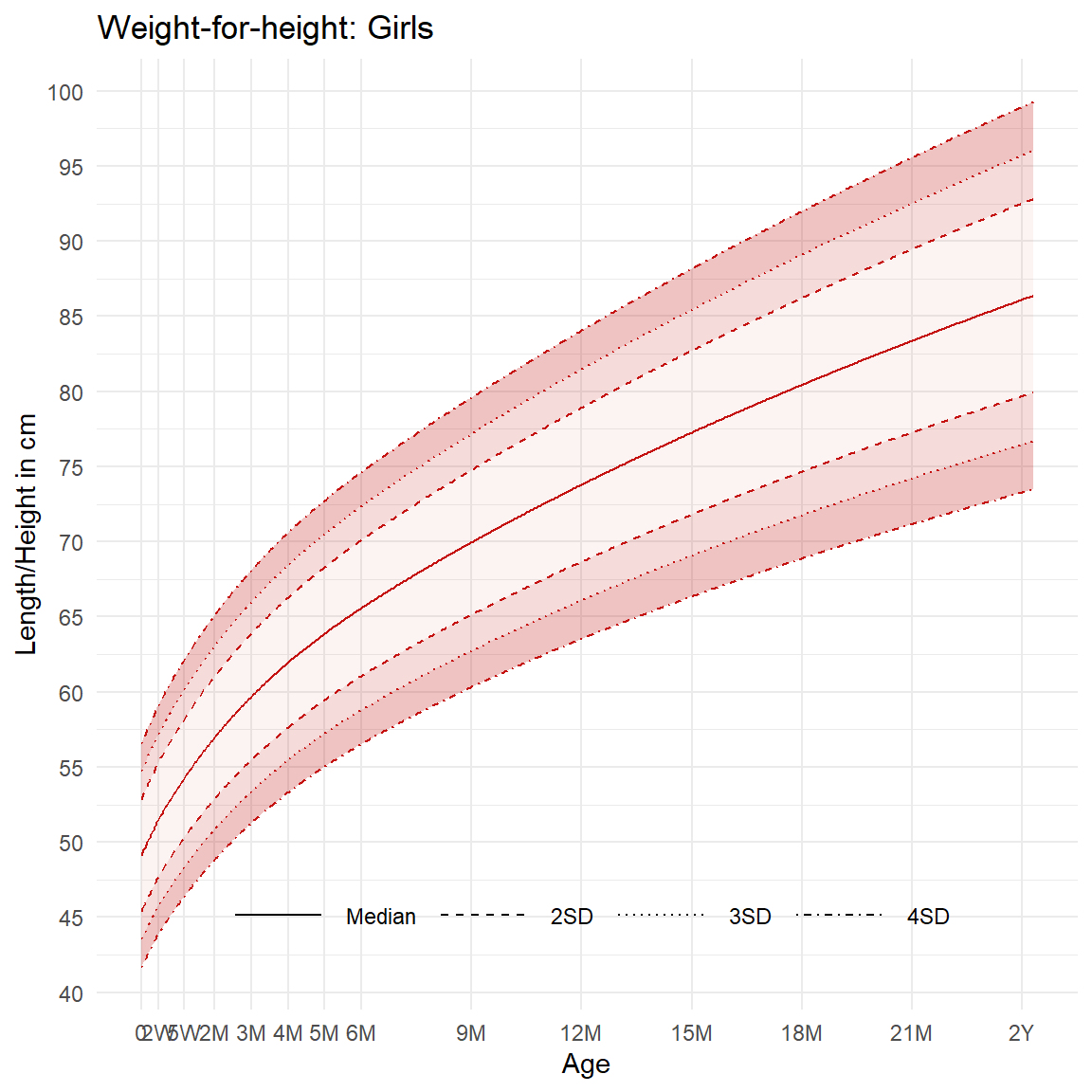
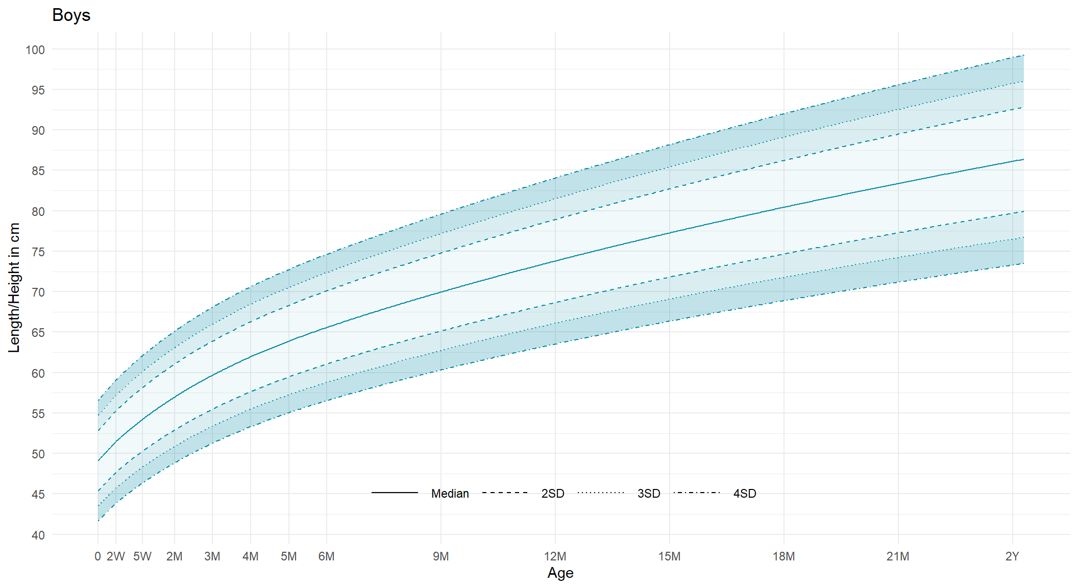
The Height-for-age standard stipulates:

• Lower boundaries of heights without stunting
• at all ages 0 days - 12 years.

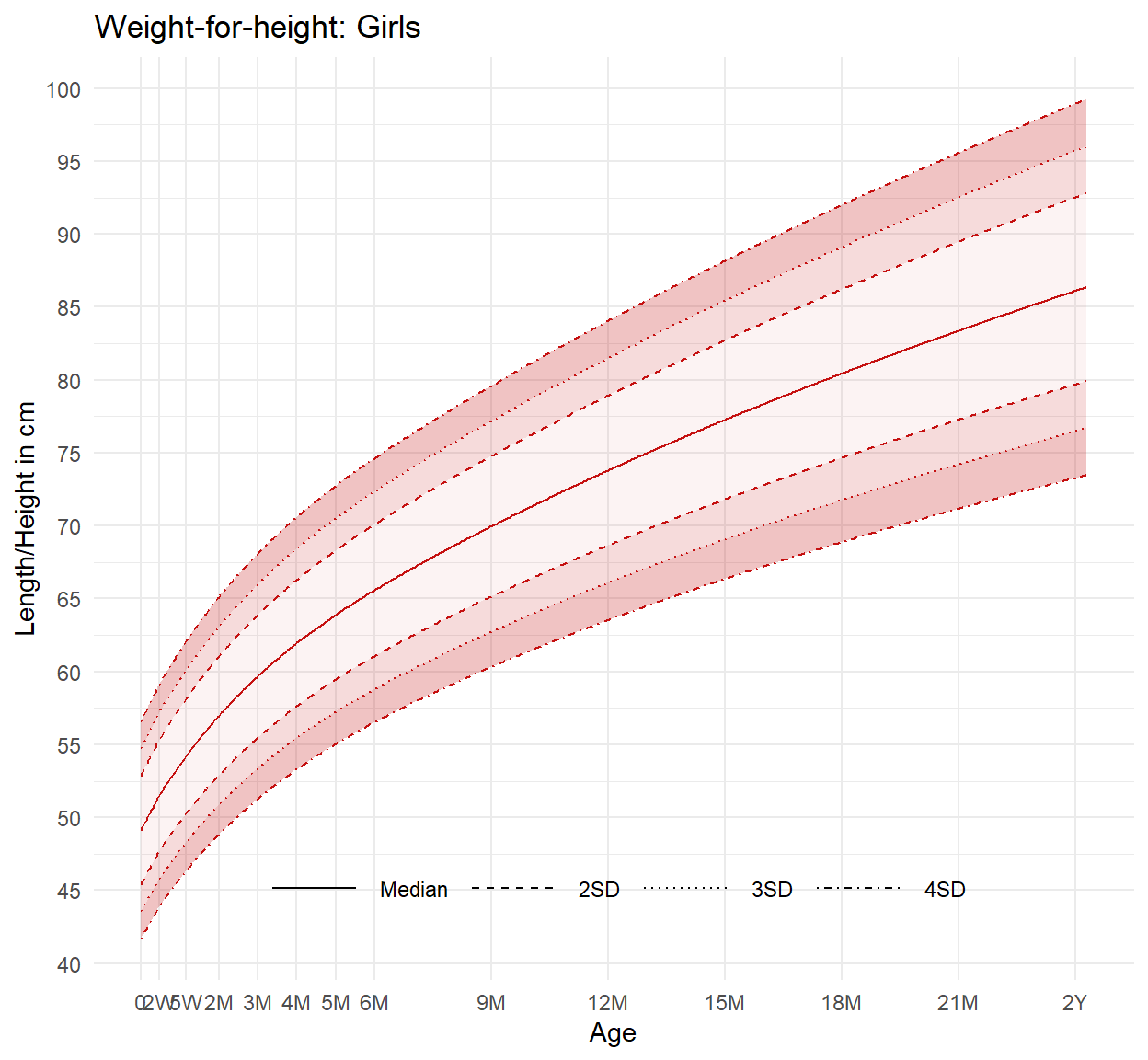
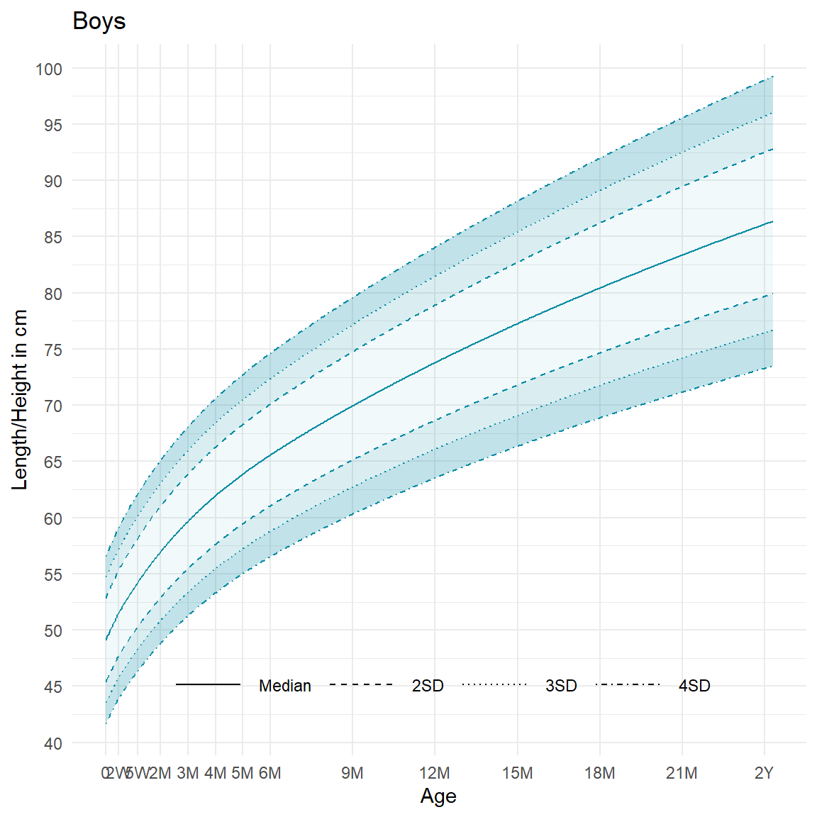
Length/Height-for-age in boys and girls

How this standard is made?

WHO’s data collection:

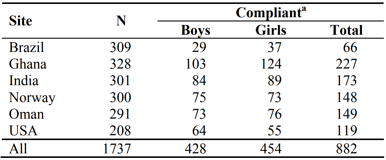
WHO Child Growth Standards

• Random sample of children was followed in each country for several years.

• Children were regularly screened and measured.

Simplified methodology:

For every age group:

• Mean/median and standard deviation were calculated.

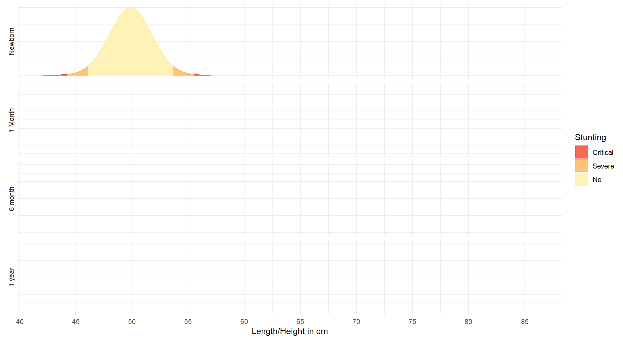
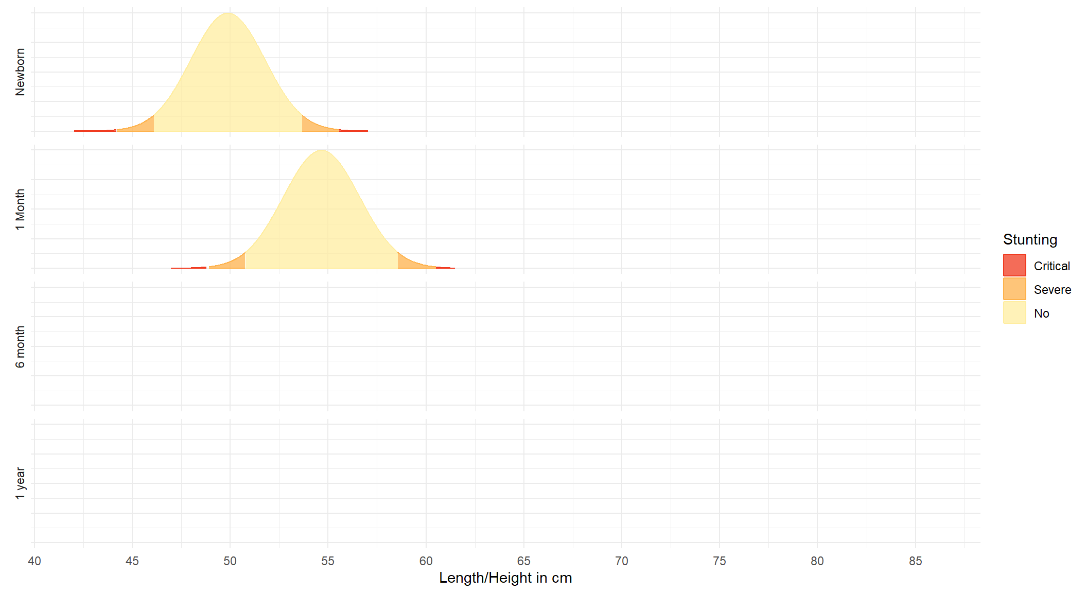
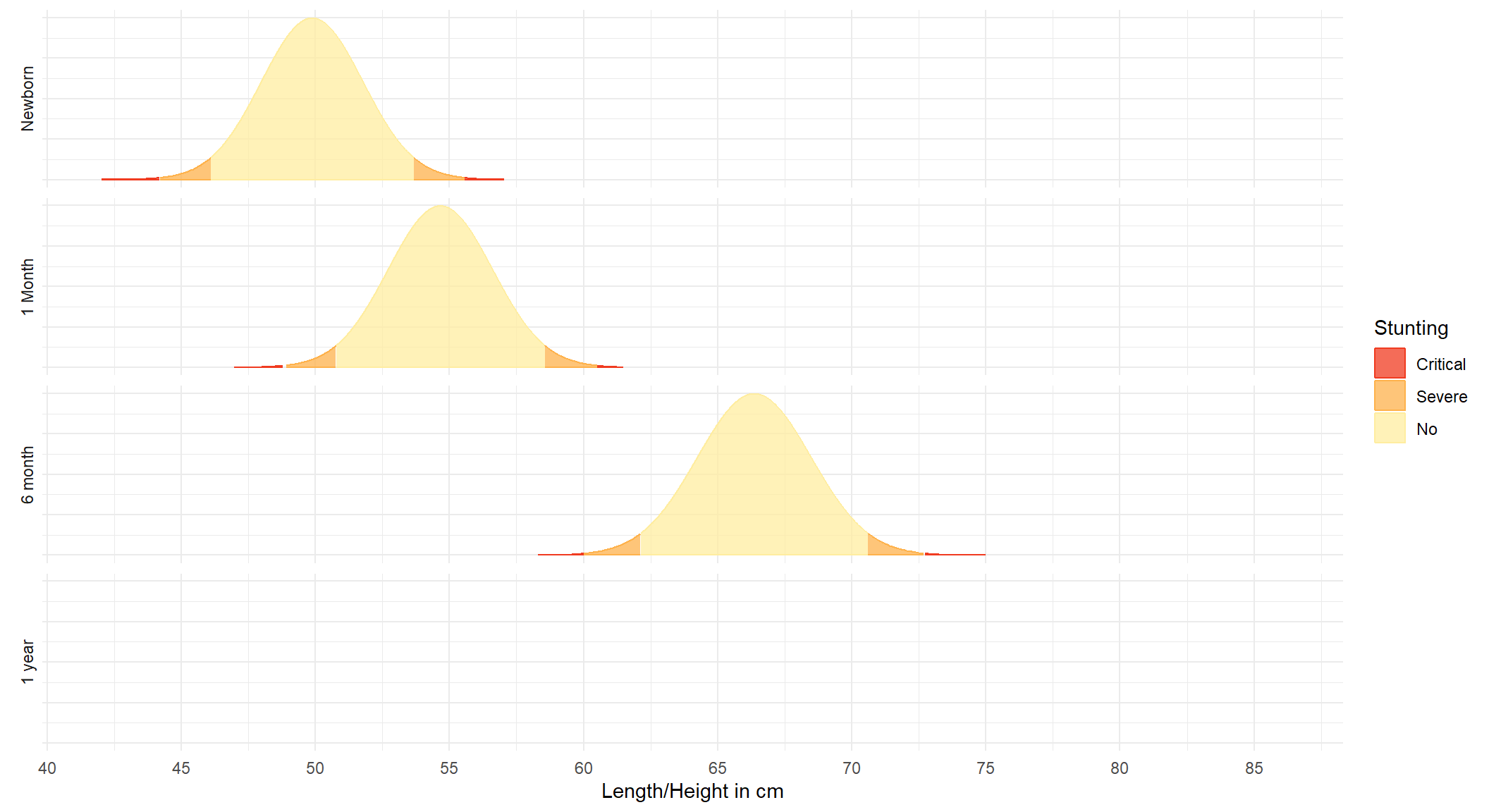
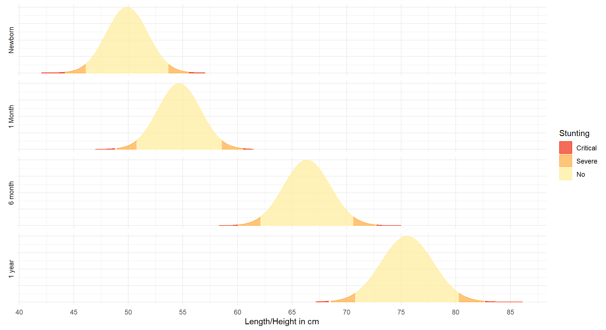
• Any child with height-for-age within two standard deviations from the mean is considered non-stunting.

• For a regular population, 95% of children are not stunted.

How this standard is made?

The stanard summary

WHO’s data on the healthy population defined

• probability distributions of heights for age and gender of children

by:

• Calculating mean, height at age and its standard deviation

• Assuming that the distribution is normal

Stunting was defined as:

• actual height 2 standard deviation below the mean of a healthy population.

Application: let us follow a boy’s development:

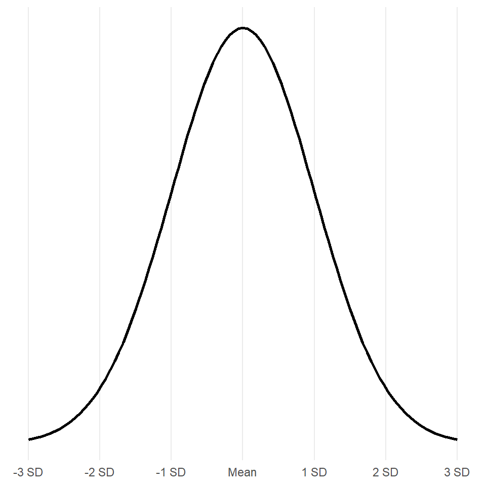
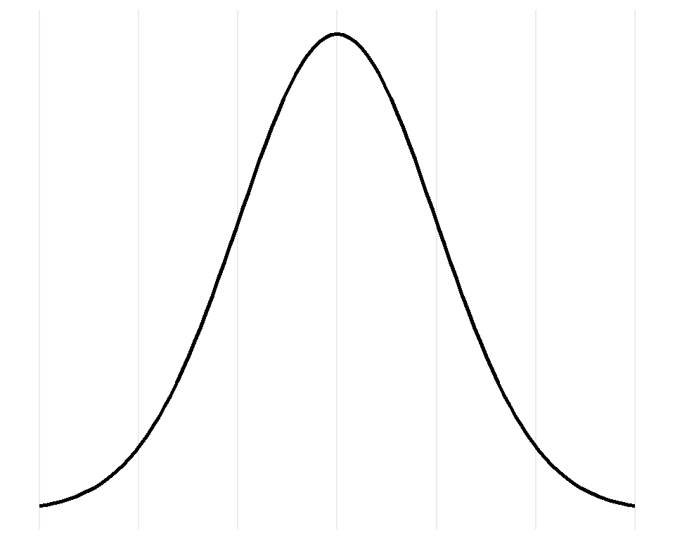
The (Satandard) Normal Distribution

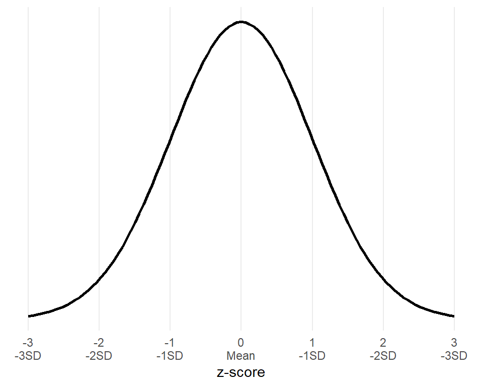
Is the symmetric, bell-shaped normal distribution, whit:

• \(\mu = 0\),

• \(\text{SD} = 1\).

• X axis corresponds to the z-scores.

Z-score

The Z-score of an observation \(x_i\) is the number of standard deviations \(s\) that it (\(x_i\)) falls above or below the mean \(\bar x\).

We can compute a z-score of every observation \(x_i\) in our sample. For that we need:

• sample mean \(\bar x\), and
• sample standard deviation, \(s\).

\[ Z_i = \frac{x_i-\bar x}{s} \]

Please memorize it!

Why do we need it?

• to compare distributions, or
• locate an individual observations \(i\) on / relative to a distribution.
• to determine % of population below and above such an observation \(i\)

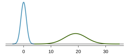
Standardization

The process of converting any value \(i\) of any distribution to a standard normal distribution.

\[ Z_i = \frac{x_i - \bar x}{s} \]

where:

• \(\bar x\) is the mean, and
• \(s\) is the SD, and
• \(x_i\) is the observation \(i\).

Example (exam): det. stunting status (1)

Stunting is defined as having height 2 standard deviations lower then the average height of a healthy child of the same gender and age.

We’ve measured that:

• a 5 years old girl is 97 cm tall

Can we consider her suffering from stunting?

According to the Child Growth Standards about height-for-age, the height of a healthy girl at the age of 5 years old:

• is normally distributed with
• the mean \(\mu = 109\) cm and
• the SD \(s = 4.73\) cm.

Example: determine stunting status (2)

Computing the z-score of the observation:

\[ Z = \frac{97 - 109}{4.73} = \frac{-12}{4.73} = -2.54 \]

Conclusion:

• Observed height of a 5 y.o. girl falls below -2 standard deviations.

• Thus she might be suffering from stunting if other causes of growth deprevation (e.g. genetic) are eliminated.

When univariate data analysis is not enough?

Datasaur: Synthetic data (1)

• There are 13 synthetic data sets that produce similar descriptive statistics and distributions:

dataset	mean_x	mean_y
away	54.27	47.83
bullseye	54.27	47.83
circle	54.27	47.84
dino	54.26	47.83
dots	54.26	47.84
h_lines	54.26	47.83
high_lines	54.27	47.84
slant_down	54.27	47.84
slant_up	54.27	47.83
star	54.27	47.84
v_lines	54.27	47.84
wide_lines	54.27	47.83
x_shape	54.26	47.84

Univariate analysis of the Datasaur (1)

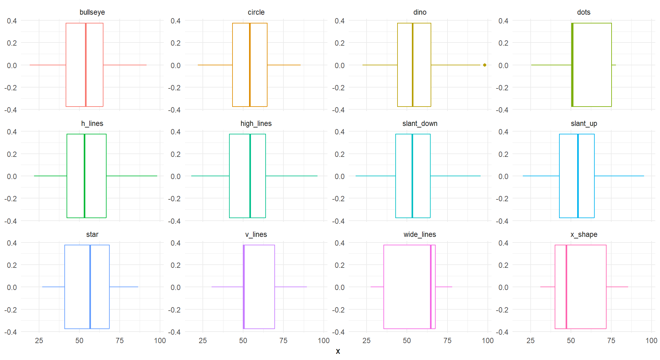
Univariate analysis of the Datasaur (2)

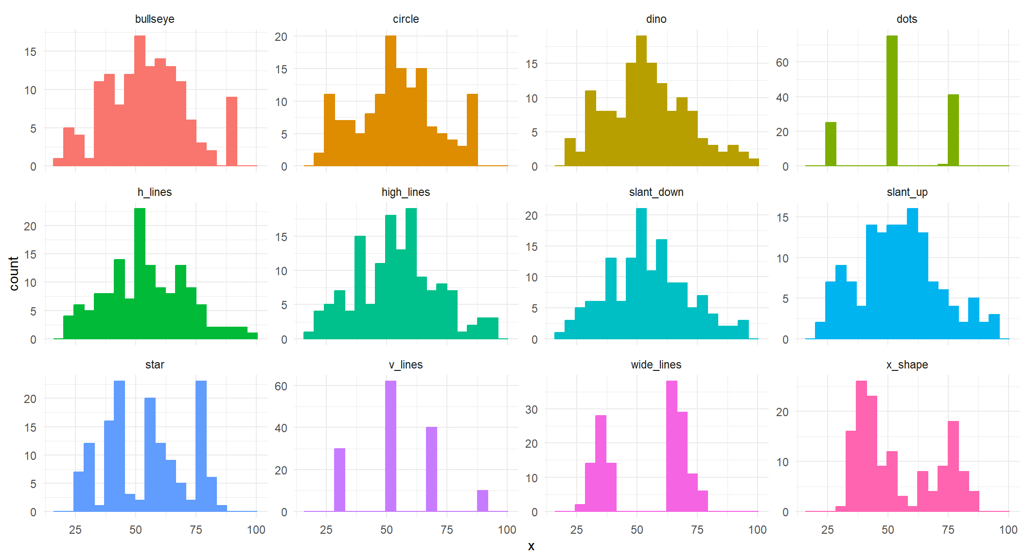
Bi-variate distribution is important!

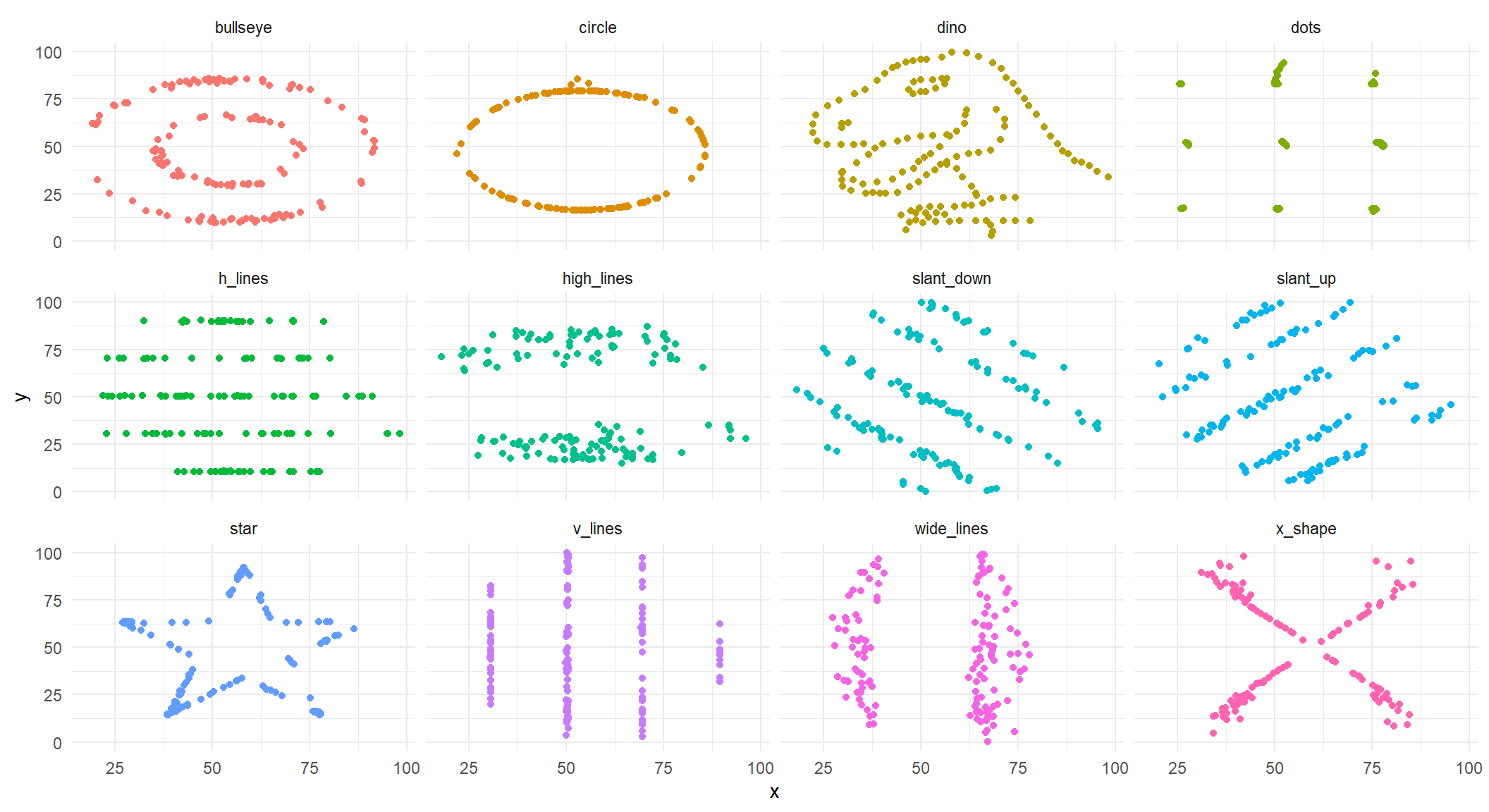
Read before week 4!

• Chapter 1 Randomized Trials. In Mastering ’metrics : the path from cause to effect / Joshua D. Angrist and Jörn-Steffen Pischk. Princeton University Press, 2015. https://justfind.hds.hebis.de/Record/HEB35797798X

• Available online / library

Homework examples

Compute z-score

1. The boy’s height is 76 cm. He is 1.5 Years old.

   • Is this boy stunted given that the expected height in the corresponding population of that age is 80.3 and the SD is 2.6?
   • Calculate corresponding statistics and write a brief conclusion.

2. The girl’s weight is 13.8 kg. She is 5 years old.

   • Does this girl suffer from waisting?
   • Expected weight in the corresponding population of that age is 18.3 and the SD is 2.05?
   • Calculate corresponding statistics and write a brief conclusion.

Exam questions on variance

• What is variance and how is it different from the standard deviation.

• When the mean and the standard deviation are not the best measures of respectively the central tendency and the variance?

  • What are the alternative methods?

• Assume that the distribution is normal. What share of observations falls withing two SD of mean?

• How the quantiles are constructed?

• Is median one of the quantiles or this is the central tendency?

• What robust measures of variance do you know?

Exam questions on the Normal distribution

• What is the difference between a normal distribution of age and a standard normal distribution?

• What is the z-score?

Takeaways checklist

Read more about income inequality at Our World in Data

• The history of global economic inequality

• Global Inequality of Opportunity

• Global economic inequality: what matters most for your living conditions is not who you are, but where you are

• Income inequality before and after taxes: How much do countries redistribute income?

• OWID Data Collection: Inequality and Poverty

• How has inequality in the United Kingdom changed over the long run?

• How unequal were pre-industrial societies?

• How has income inequality within countries evolved over the past century?

Key concepts covered in the lecture

Univariate data

The Histogram:

• bars, frequencies, bins and bins width;

The Density plot:

• Density vs frequency;
• How to make a density plot;

The Cumulative distribution:

• How to make it;
• Equal vs unequal distribution;
• Lorenz Curve;

The Variance:

• Robust vs non robust statistical measures of variance;
• Variance and Standard deviation;
• Use of SD;
• Units of measurement in SD;
• 1, 2, 3 SD from the mean/median;

The Normal Distribution:

• Mean and Variance in the Normal distribution;
• Standard normal distribution;
• Z-scores and standardization;

References

Cairo, Alberto. 2016. Download the Datasaurus: Never trust summary statistics alone; always visualize your data. http://www.thefunctionalart.com/2016/08/download-datasaurus-never-trust-summary.html.

Diez, David, Mine Cetinkaya-Rundel, and Christopher D Barr. 2022. OpenIntro Statistics: Fourth Edition. OpenIntro. https://www.openintro.org/book/os/.

Dowdy, Shirley, Stanley Weardon, and Daniel Chilko. 2004. Statistics for Research. John Wiley & Sons, Inc. https://doi.org/10.1002/0471477435.

Matejka, Justin, and George Fitzmaurice. 2017. Same Stats, Different Graphs: Generating Datasets with Varied Appearance and Identical Statistics through Simulated Annealing.

Todaro, Michael, and Stephen C. Smith. 2014. Economic Development. 11th ed. Pearson.

Wilke, Claus O. 2019. Fundamentals of Data Visualization: A Primer on Making Informative and Compelling Figures. O’Reilly Media.